What follows is an essay adapted from a talk, delivered in 2010 to teenagers and parents in my hometown of Cupertino, California. The talk concerned the surfaces of things, like bodies and planets, and abstract surfaces, like the Möbius strip and the torus. The goal was to learn about the world by studying surfaces mathematically, to learn about mathematics by studying the way we study surfaces, and, ideally, to learn about ourselves by studying how we do mathematics.
Imagine that you are an emperor regarding a great expanse from a tall peak. Though your territory extends beyond your sight, a map of the entire empire hangs on the wall in your study, seventy interlocking cantons. On your desk lies a thick, bound atlas. Each page is a detailed map of a county whose image on the great map is smaller than a coin.
You dream of an atlas of the world in which the map of your empire would fill but a single page. You send forth a fleet of cartographers. They scatter from the capitol and each, after traveling her assigned distance, will make a detailed map of her surroundings, note the names of her colleagues in each adjacent plot, and return.
If the world is infinite, some surveyors will return with bad news: they were the member of their band to travel the furthest and uncharted territory lies on one side of their map. But if the world is finite, there will be many happy surprises: a friend last seen in the capitol is rediscovered thousands of miles from home, having taken another path to the same place. Their maps form an atlas of the world.
You have another dream, in which the whole world is contained in your capable hands, miniature and alive. Upon waking, you begin to tear the pages out of the atlas and piece them together, using the labels on the edge of each page to stitch it to its neighbors, constructing ever larger swaths of territory.
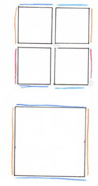
Soon you are left with six grand charts. You fit them together and they lift off the table to form a cube.
![]()
An atlas of squares assembles into a cube.
You are perplexed. Can the world have creases and corners? If smooth skin is cut and then sutured, a ridge of stitches shows. Perhaps the sharp edges come from the mapping not the land. You suddenly recall the map of your own canton, centered on the mountain on which you live. If a mountain can be flat on a map, perhaps a peak on a map can represent flat land. Some distortion must be inevitable in this process of turning land into paper. The world might be smoothly curved, the folded map having flattened some parts and extended others.
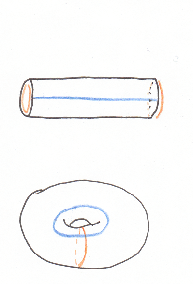
Perhaps instead you are left with four grand charts. You fit them into a larger square, then the square into a cylinder and stretch its ends to meet. The world is shaped like a tremendous torus, the surface of some heavenly wheel.
![]()
![]()
Another atlas of squares assembles into a torus.
You, dear reader, are not an emperor (yet). If you want to recover the shape of the world, you cannot send forth thousands of surveyors. But you can put yourself in his place, at the moment when the completed atlas of the world lies on his desk. You can imagine piecing it together, stitching pages along their indicated boundaries until they close up into a complete model of the world, its shape sitting before you.
If we, without sending out an expedition, can somehow make a classification of surfaces, a complete list of what an atlas might conceivably be stitched into, then we will have listed the possible shapes of the world. Exploration is of course necessary to figure out which surface from the list our actual world happens to be, but an abstract, mathematical classification will constrain the shape of any surface past, present, future, or fictional.
Sameness
Before embarking on the quest to classify surfaces, we should say what it would mean for a surface to be on our list. We must decide when we will say that two surfaces have the same shape.
The cartographical situation suggests some requirements for our notion of “same shape”.
- If you build reasonably accurate local maps of a surface and then assemble them faithfully, the resulting paper model has the same shape as the original surface.
- If you deform a surface slightly, say through the erosion of a mountaintop, then its shape does not change.
While these conditions sound innocuous, they have some strange ramifications.
Say you begin with a ball of clay. Its surface is a sphere. You toss it on a potter’s wheel, flattening the base a bit. As the wheel spins, you press on the sides, then depress the center, then squeeze the walls you have formed a bowl. Since each change was so mild, you must never have changed the fundamental shape of the object.1 We must say that the surface of a ball is the same shape as the surface of a bowl.
The branch of mathematics concerned with the study of shape and space is called topology (from ancient Greek topos, meaning place). An oft-repeated and never funny joke is that a topologist cannot tell a coffee mug from a donut. This is not true. But it is true that mathematicians abstract the sensory qualities from a thing (the heft of the mug, the sweetness of the donut). And if both mug and donut were made of a perfectly malleable substance, you might expand the base of the mug to fill up its volume, then shrink the resulting thick cylinder down until it's the same width as the handle, leaving a torus. It’s not that topologists think it desirable that a donut be a coffee mug. It’s that, having promised to allow small deformations and being honorable folk, they are obligated to admit that the mug and donut have the same shape. 2
The topological notion of “same shape” can actually be defined in terms of maps. Two surfaces A and B have the same shape if you can draw a faithful map of A on B. In other words, there is a continuous correspondence between the points of A and the points of B--an assignment to every point of A exactly one point of B in such a way that any smooth path you draw between two points on A maps to a smooth path on B, and vice versa.
(In this sense, the Mercator projection is not a map of the earth. To begin with, two points, the North and South poles, are missing entirely. Moreover, on the real earth one can sail from San Francisco to Japan through the Pacific. On the Mercator projection, the ship hits the edge of the map.)
If you start with a object and deform it, squeezing, pinching, pulling, etc, then whatever you end up with comes with a map already made: the surface of the original lies distorted on the final product. While the earth (unbeknownst to our emperor) is not a perfect ball, its surface not a perfect sphere, they are, topologically, the same shape: push in the mountains, pull out the valleys, smooth it out.
We can now compare physical surfaces to infinitely thin abstract ones. We can jump scale from maps and atlases to planets—just write down a correspondence of points. Consider the emperor's cube stitched together out of the atlas's pages. Place it at the center of a Japanese lantern, a thin white paper sphere, with a very bright light inside the cube. The projection is our one-to-one correspondence, the image of the cube exactly covers the sphere; the cube is the same shape as the sphere.
Difference
Under the topological definition of sameness, it is easy to verify that two surfaces are the same but hard to demonstrate that they’re different. How could we prove that no possible correspondence can exist between two surfaces? If one surface fits in the palm and we live inside the other, if one is presented as pages in an atlas and the other as a habitat, we might have to be rather clever to find the right correspondence. We need an invariant, something which can be computed about a surface that doesn't depend on how it's presented to us, something that can prohibit the existence of any continuous correspondence and tell us: these really are different.
A first difference: the disk is not the sphere. Why? The disk has a boundary, an edge, and the points on the edge are special. To see this, imagine yourself living in the surface. Imagine that the thin surface is sandwiched between two sheets of glass, and you are a paramecium, a single-celled organism swimming sideways. When you come to an edge, you have to stop--points on the boundary of the disk have the special property that some directions of travel are forbidden. At every point of the sphere, however, you have a full range of motion. There can be no continuous correspondence between the disk and the sphere because the point on the sphere ending up on the boundary of the disk would have to be ripped away from its neighbor. Tearing is very discontinuous.
This gives us our first invariant, the number of components in the boundary of a surface or the number of holes it has cut into it. The location of the holes doesn’t affect the shape, since we could shrink them to pinpricks then slide them to any other location on the surface. A sphere with two holes at opposite poles is the same shape as a sphere with two holes next to each other is the same as a hollow tube.
We can also distinguish finite surfaces from infinite surfaces like the vast plane that Euclidean geometry takes place on. We're assuming that all the surveyors returned with good news, so the theoretical earth we're trying to map is finite.
In addition to asking about a surface, “does it have boundary?” or “is it finite?” we can ask, “is it orientable?” The extrinsic definition of orientable applies to a surface that you're handed, sitting in 3 dimensions (as opposed to an atlas with identifications), the kind of surface you can jump off of. It's orientable if it has two sides (like the sphere), which we usually call the in-side and the out-side. It's nonorientable if it has only one, like the Möbius strip.
We can also define orientability intrinsically, for people who live in the surface, not on it. People like our paramecium. Let’s call him TK. Imagine that TK’s little cilia spin clockwise, giving his body a preferred direction of rotation, and that he has an identical twin JW. Now TK can wander around through the surface, taking some convoluted path, then return to where he started. For many paths, he still looks like JW upon his return, cilia twisting clockwise. But maybe he comes back reversed, cilia twisting counterclockwise--this is exactly what happens in the Möbius strip. If there is a path TK can take and come back reversed from his twin, then the surface is nonorientable. Otherwise, it's orientable. This implies the extrinsic definition by the right-hand rule.
The surfaces of things, of thick 3-dimensional bodies, are necessarily orientable. The body itself defines the inside, which cannot be reached traveling on the outside. Surfaces of things are also finite, and have no boundary--if you try to cut a hole in the surface, you just make a depression extending the surface inwards. So to classify surfaces of things, like possible shapes for the earth, we need only consider closed, finite, orientable shapes, like the sphere and the torus.
To distinguish the sphere and the torus, we need a more sophisticated invariant called the Euler characteristic. To define it, we'll take a brief digression into graph theory.
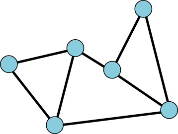
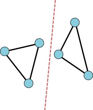
A graph is a bunch of vertices connected by a bunch of edges.
![]()
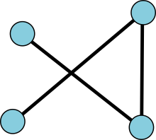
We will ask that our graph be connected, so it can't be split into two disconnected pieces. We will also ask that the graph be planar: edges don't cross. They only meet at vertices.
![]()
![]()
Disconnected graphs are forbidden. Edges should not cross.
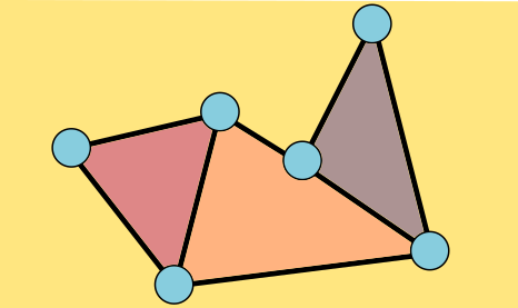
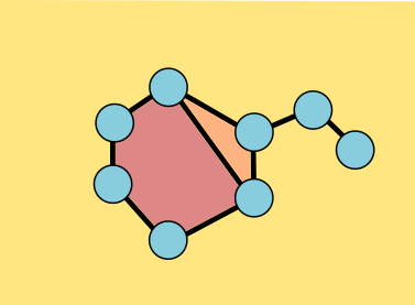
On a planar graph, we can also count faces. Those are the regions of the plane bounded by edges, the areas that would get colored in MS paint if you put the little paint bucket over them and clicked. The outside counts as one big face, since when you click, it's colored.
![]()
This graph has 6 vertices, 8 edges, and 4 faces. Its Euler characteristic is 2.
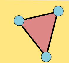
The Euler characteristic of the graph, which I'll denote χ, is the number of vertices minus the number of edges plus the number of faces, which is here 6 – 8 + 4 = 2. The Euler characteristic of triangle is easy: 3 - 3 + 2 = 2.
![]()
![]()
Theorem: The Euler characteristic of a connected planar graph is always 2.
Proof: Start drawing the graph. We begin with a single vertex and the single big face, χ = 1+1 = 2. We add a vertex, and to keep the graph connected, we add an edge. Plus 1, minus 1, χ is still 2. Add a few more vertices, each with its edge, and χ stays the same. What else can happen? We can add an edge connecting two vertices already drawn. That edge will split an existing face into two, creating another face, and preserving χ. Another edge, another face, same χ. We build up the graph from a single vertex. χ starts at 2, and every additional vertex comes with an edge, fixing χ, and every solo edge comes with a face, fixing χ. So when we've drawn the whole graph, χ is still 2. Every connected graph in the plane has Euler characteristic 2. This was a proof by induction.
![]()
As a graph grows, its Euler characteristic remains constant.
The same equality holds on the sphere, and we have actually proved it already. Draw the graph near the top of the sphere and the outer face from the plane will become the bottom face on the sphere. We also have a bunch of graphs on the sphere readymade for us: the Platonic solids. On the emperor's paper cube with the bright light inside, the dark edges of the cube project a graph on the sphere, a graph with eight vertices, twelve edges, and six faces: χ = 8 - 12 + 6 = 2. All the other Platonic solids, when projected onto the sphere in the same way, give graphs. An exercise for the reader: check that the Euler characteristic of each of those graphs is 2.
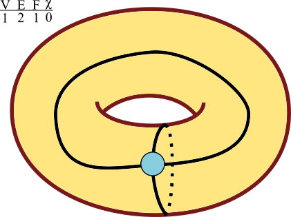
What about graphs on other surfaces, like the torus? If we start with a single vertex, χ is 2, one vertex one funny shaped face. But if we add a self-edge wrapping around, then χ is 1, and we still have one face, which is now shaped like a cylinder. We can add one more edge without changing splitting the face, lowering χ to 1 - 2 + 1 = 0. From now on, though, the same induction works. Every face is a polygon, and every additional edge splits a face, and χ is always 0.
![]()
A graph on the torus has Euler characteristic 0.
We can now prove that the sphere is topologically different than the torus! For suppose we had a continuous correspondence between the two. It would take this connected graph on the torus, with χ = 0, to some graph on the sphere. Since the map corresponds single points to single points, edges which don't cross on the torus will not cross on the sphere, and the graph will still be planar. Same number of vertices, same number of edges, same number of faces--same graph! So same χ. But χ of any graph on the sphere is 2. So there can be no continuous correspondence between the sphere and the torus--they are topologically distinct surfaces, with different shapes.
It turns out that when you start drawing any graph G on the torus, once every face is a polygon, χ stays the same. This condition came for free on the sphere, where the big face starts out as a disk. In fact, χ always stabilizes at 0. To see this notice that we could add extra edges and vertices until our graph G’ contains a copy of the simple graph S with one vertex and two self-loops. This graph could also be built by starting with S and adding edges too; as a descendent of G and of S, it has the same Euler characteristic as both of them. Since χ(S) = 0, χ(G’) and χ(G) are 0 too. Any graph with polygonal faces on the torus has Euler characteristic 0.
Classification
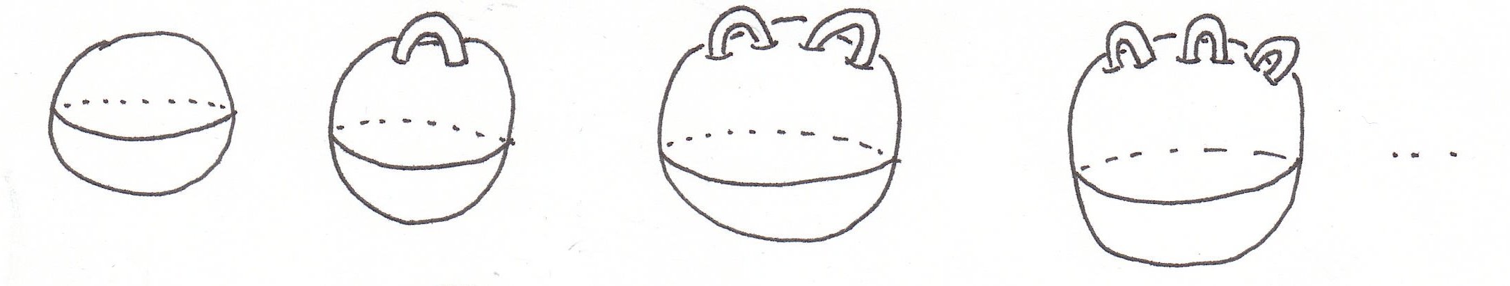
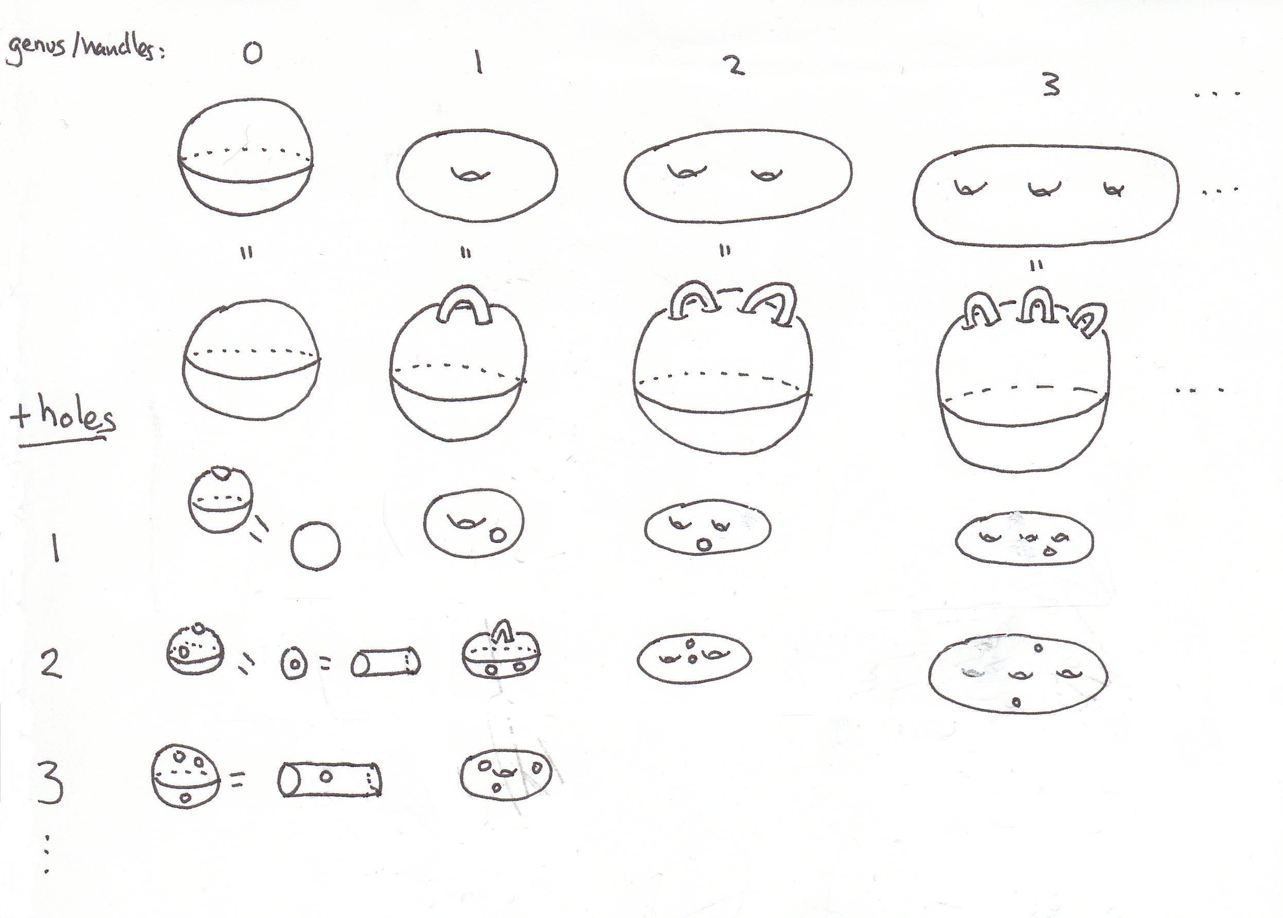
The time has come to classify surfaces. First we make a list of boundary-free orientable surfaces: start with a sphere and add handles. Ball, kettlebell, etc. Soon we will show that this is the list.
![]()
Of course the torus is on the list. It has the same shape as a sphere with a handle attached--shrink the sphere until it's the same size as the handle. In fact, all the closed surfaces we have seen have the shape of a sphere with handles. The number of handles is called the genus of the surface.
It is possible to define the Euler characteristic for graphs on any surface. As long as all the faces of a graph are polygons, then count χ = V – E + F depends only on the shape of the surface. A sphere has χ = 2, a sphere with one handle has χ = 0, a sphere with two handles has χ = -2, a sphere with g handles has χ = 2 - 2g. This proves that all of the closed, oriented surfaces on our list are distinct; we're not double-counting.
We want to prove that our list of possible shapes for the surface of the earth is complete. As is often the case in mathematics, it’s actually easier to prove something more general. We will classify all finite orientable surfaces, including those with boundary.
![]()
Theorem: Every finite, orientable surface has the shape of a sphere with handles, possibly with holes.
Proof: We can assume that the atlas gathered by our surveyors has triangular pages--any other shape (e.g. a square) can be further cut up into triangles. We will build our world by stitching together the pages of the atlas along the identifications marked by the surveyors. The plan is to show that at every stage of this construction, our world-in-progress is a surface on this list. This is a proof by induction, like our proof of the invariance of the Euler characteristic. This will be a sketch, so don't worry too much if a step seems a bit sketchy--the geometric imagination required to follow proofs like this is an acquired skill.
The base case is easy: we start with a single triangle, which is topologically a disk, or a sphere with one hole in it. When we add a second triangle, if we just stitch one side of the new triangle on, the topology doesn't change. Stitching together the sides of two adjacent triangles also keeps the shape the same.
![]()
If we attach all three sides, then we're filling in a hole: sphere with one hole closes off to form a sphere with no holes.
We're always attaching the edges of the new triangle along the boundary of our current surface. If we attach two edges of the triangle along adjacent edges of the boundary, the topology doesn't change. But if we attach two edges along separated parts of the same boundary component, the same boundary circle, then we've changed the topology. If we fill in all the holes in the surface before the addition, we must have gotten some genus g surface, some sphere with handles (by induction). If we fill in the holes on the new surface, after the addition, we get the same thing. But our new surface has an additional boundary component, a new hole--one circle was replaced by two. So we have moved to the right in our list.
![]()
The only other case we need to worry about is when we attach one edge of the triangle to one boundary circle and another edge to another. Then two boundary components turn into one long one. So, theoretically, we could stitch on a disk to close off the surface, and it should be on our list. This is harder to see, but the genus goes up by one, holes down one.
![]()
In summary, here is our proof that every compact, orientable surface (like the surface of the earth) is on our list. It can be build out of the pages of a triangular atlas. Adding a triangle either changes nothing, adds a hole, closes a hole, or adds a handle and subtracts a hole. You don't need to follow all the details, but the main idea is a good one to keep in mind: to classify something, make the list first, then try to prove that the list is closed under basic operations (here, adding a triangle).
Before closing the book on this classification, I would like to recall another one, very different in spirit:
These ambiguities, redundancies, and deficiencies recall those attributed by Dr. Franz Kuhn to a certain Chinese encyclopedia called the Heavenly Emporium of Benevolent Knowledge. In its distant pages it is written that animals are divided into (a) those that belong to the emperor; (b) embalmed ones; (c) those that are trained; (d) suckling pigs; (e) mermaids; (f) fabulous ones; (g) stray dogs; (h) those that are included in this classification; (i) those that tremble as if they were mad; (j) innumerable ones; (k) those drawn with a very fine camel's-hair brush; (l) etcetera; (m) those that have just broken the flower vase; (n) those that at a distance resemble flies. (Jorge Luis Borges, The Analytical Language of John Wilkins)
The (somewhat humorous) specificity of the items in the list of animals is striking--that color and texture, that idiosyncrasy, is precisely what we lose in the process of mathematicization. But in exchange for character and characteristic, we obtain generality and decidability. (A surface with Euler characteristic 0 clearly does not have Euler characteristic 2, but it’s less clear that a mermaid is not fabulous). Let me suggest an entertaining activity for moments you are bored or your phone is out of batteries. Look at the surface of a thing around you and morph it in your mind until you see it as a sphere with handles, until you recognize its shape and its place on the list. (A version for parties: what is the genus of the surface of the human body? Does it depend on gender?)
Our emperor, sitting at his desk awaiting the return of his surveyors knows that the shape of the world cannot but be a sphere, or a torus, etc--the imagined and the actual world are constrained to lie in this sequence.
![]()
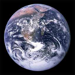
The surface of the Earth.
That emperor's thought experiment has been physically answered: with the advent of satellites, we can now apprehend the two-dimensional world we live on as the surface of a thing. But what about the three-dimensional universe we live in? If we send out surveyors from the earth in all directions, will they reencounter one another far from home?
We cannot make that voyage, though there are attempts underway to scan the radiation aftermath of the big bang for identical patches, for two directions in which we see the same thing. It also be that the universe curves back in on itself beyond the cosmological horizon, but that its farthest reaches are traveling fast enough that no astronomical survey could possibly detect it. Here mathematics can speak where physical knowledge is actually impossible--we can attempt to classify three-dimensional spaces, and our physical universe is and must be on the list. Mathematics can reach beyond the curtain of receding stars to compass the realm of universal possibilities. ![]()
1 This is known in philosophy as the Sorites paradox, or the paradox of the heap. If you begin with a heap of sand and remove grains one by one, at what point does it cease to be a heap? The mathematician’s resolution: even the empty heap, the heap with no sand in it, is a heap too.
2There is different mathematical notion of “same shape” familiar from Euclidian geometry, called “congruence” or “isometry.” There all lengths and distances must match exactly, and every slight chip or bend changes one shape into another.


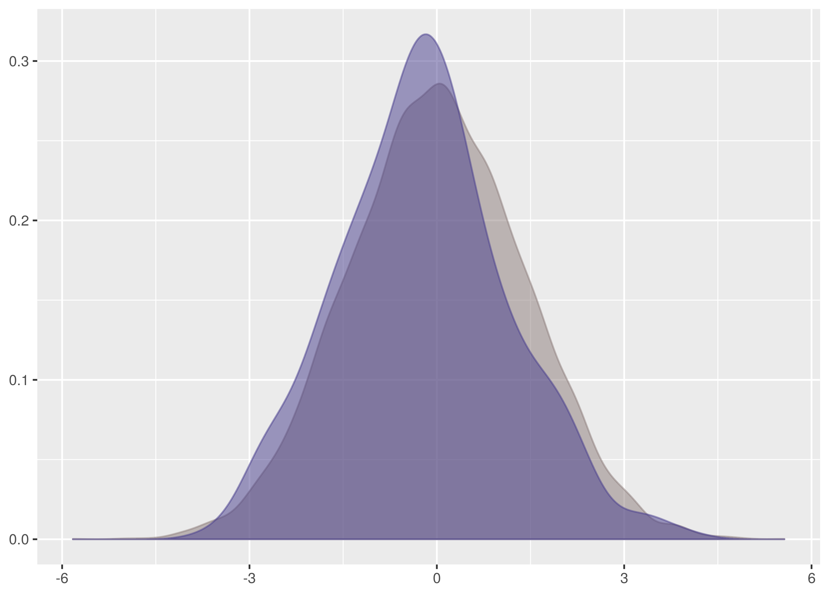
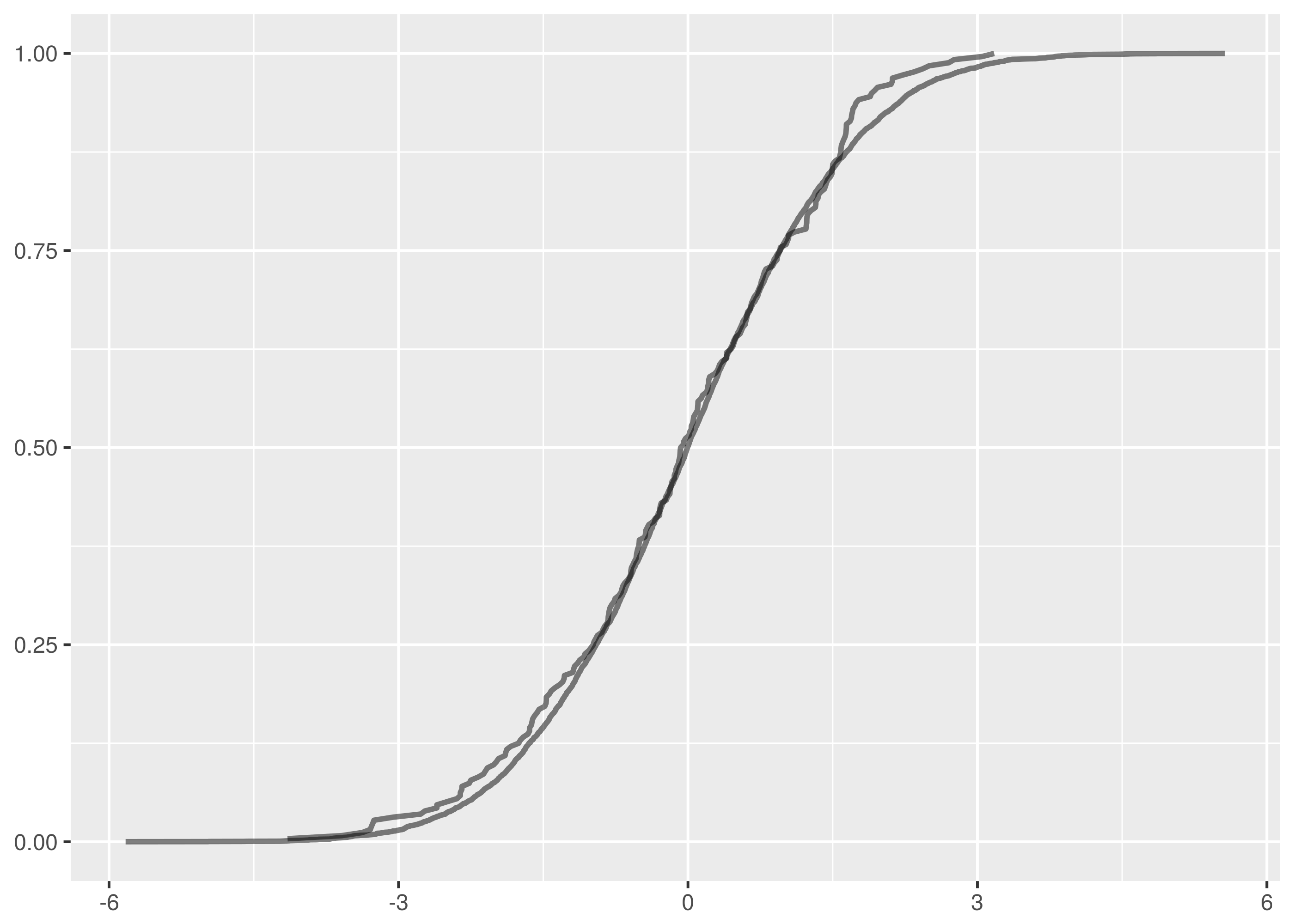
 , that the two samples we are testing come from the same distribution. Then we search for evidence that this hypothesis should be rejected and express this in terms of a probability. If the likelihood of the samples being from different distributions exceeds a confidence level we demand the original hypothesis is rejected in favour of the hypothesis,
  , that the two samples are from different distributions.
 and
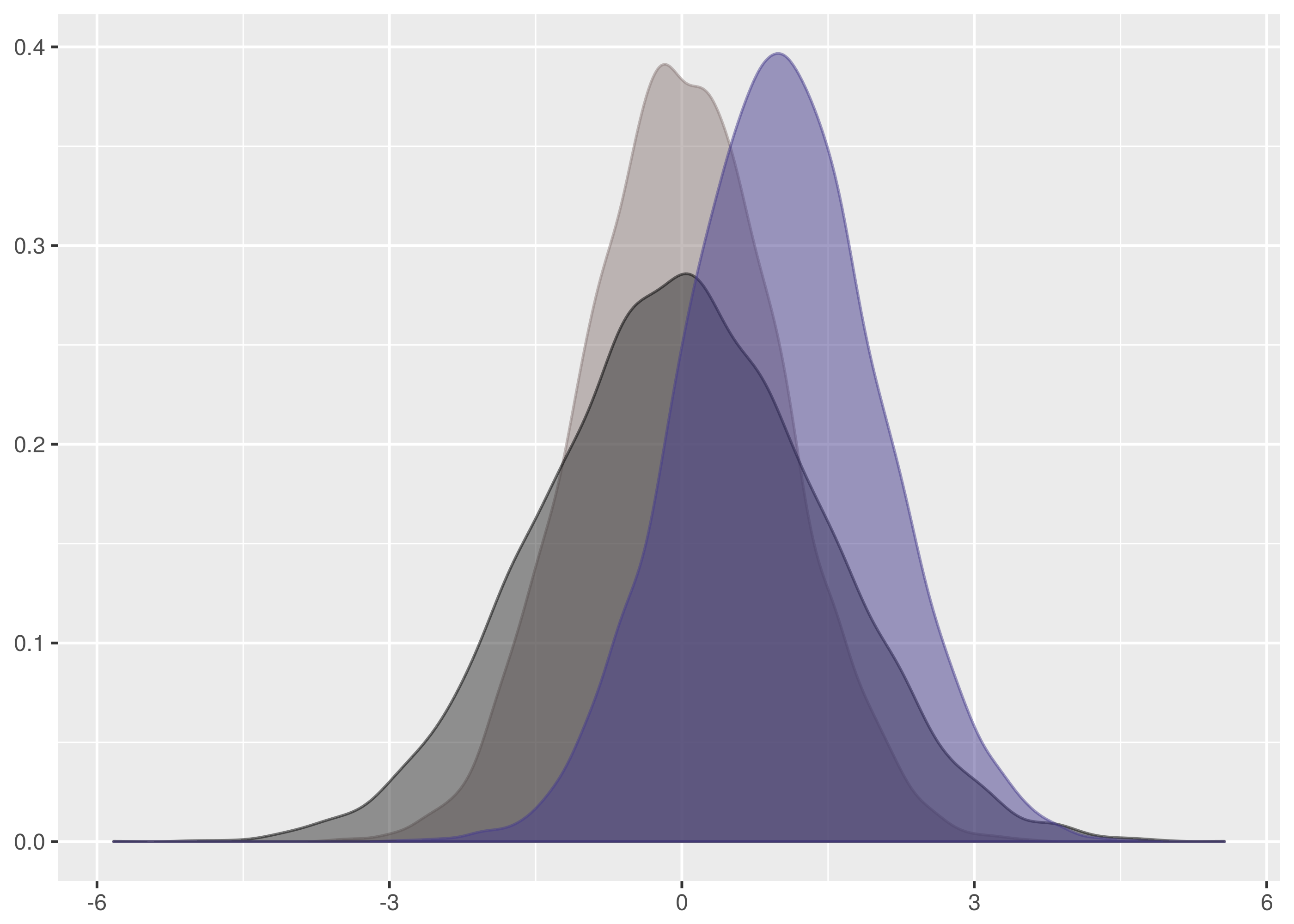
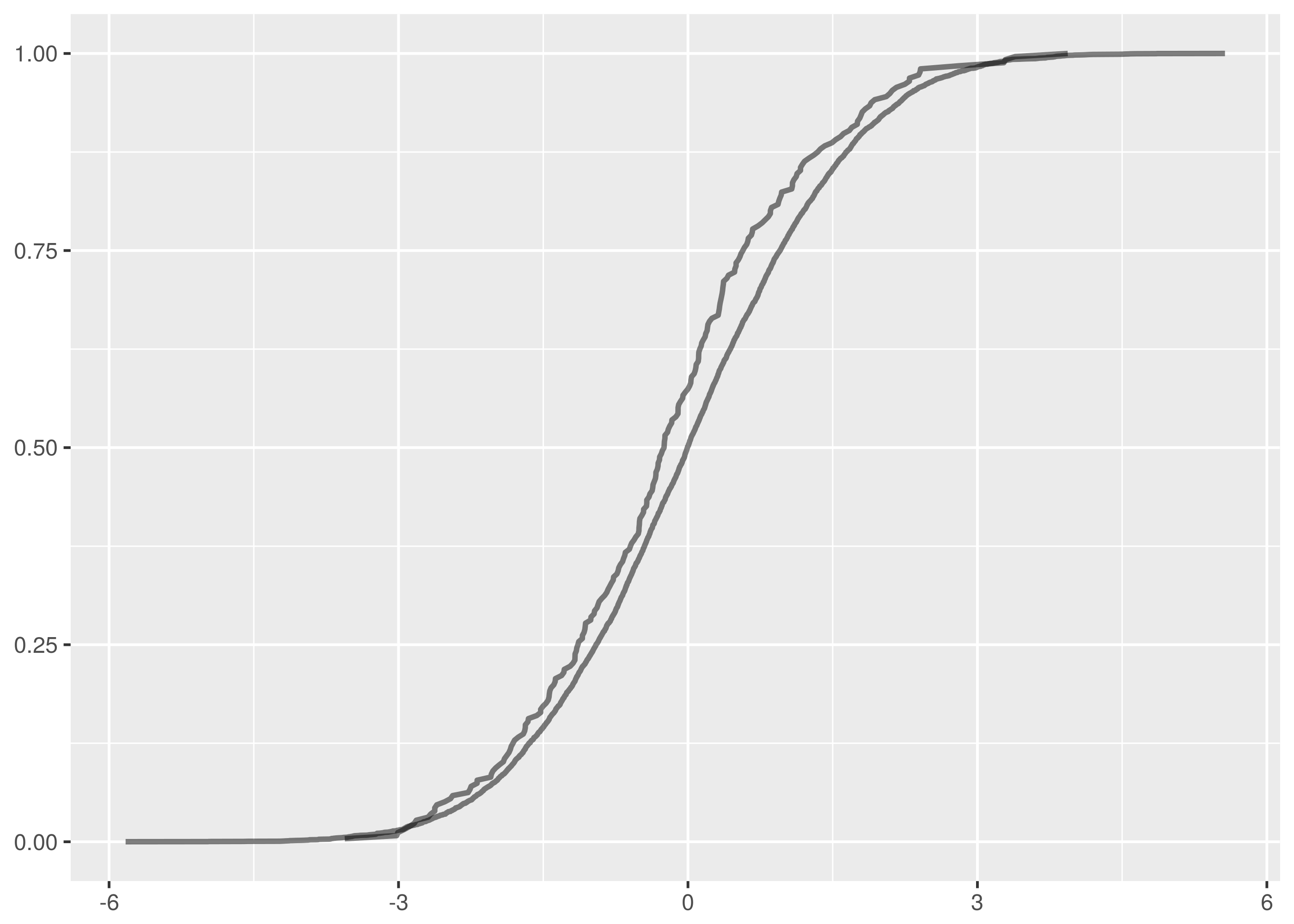
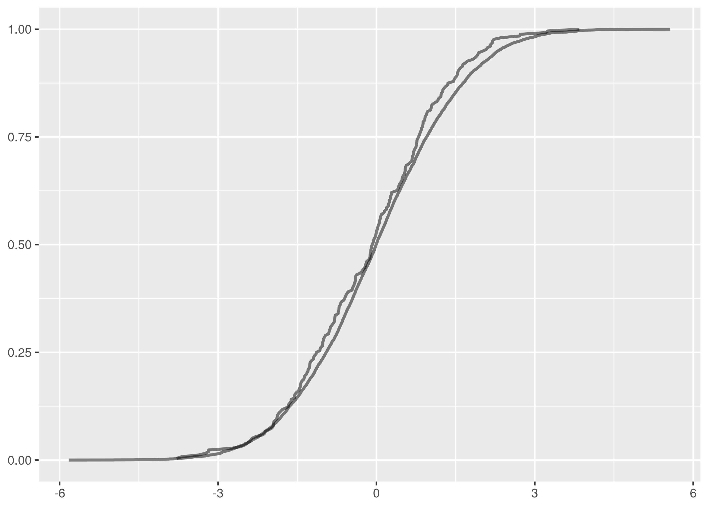
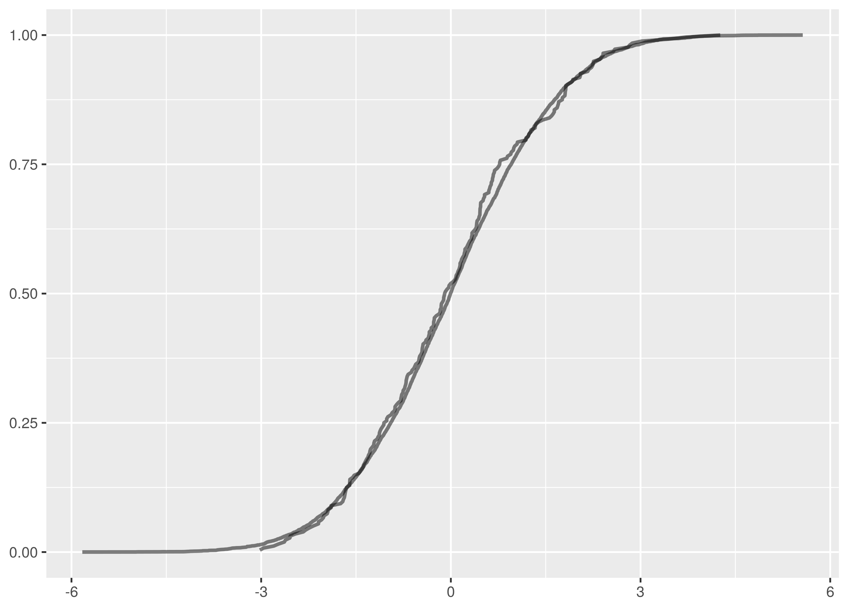
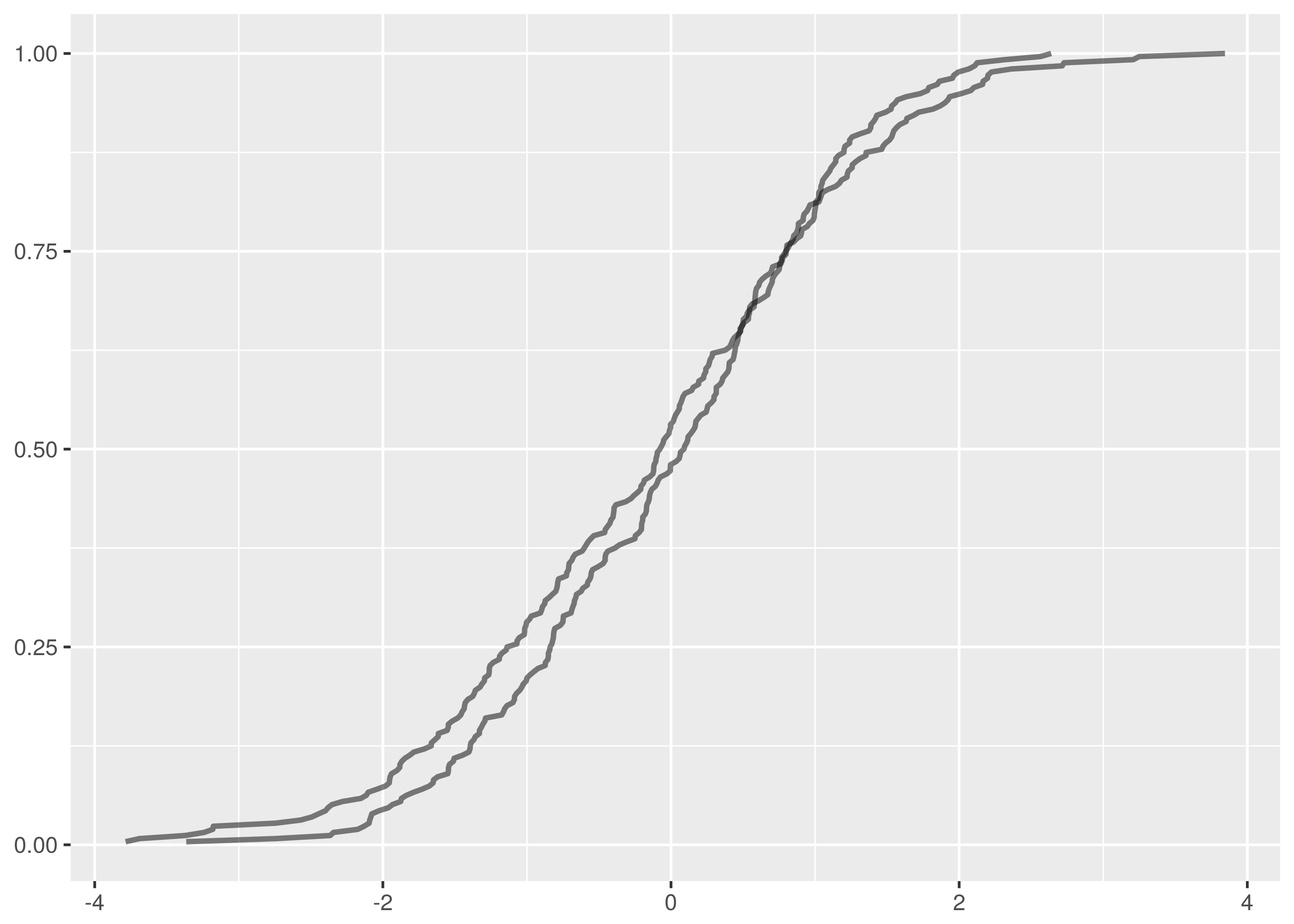
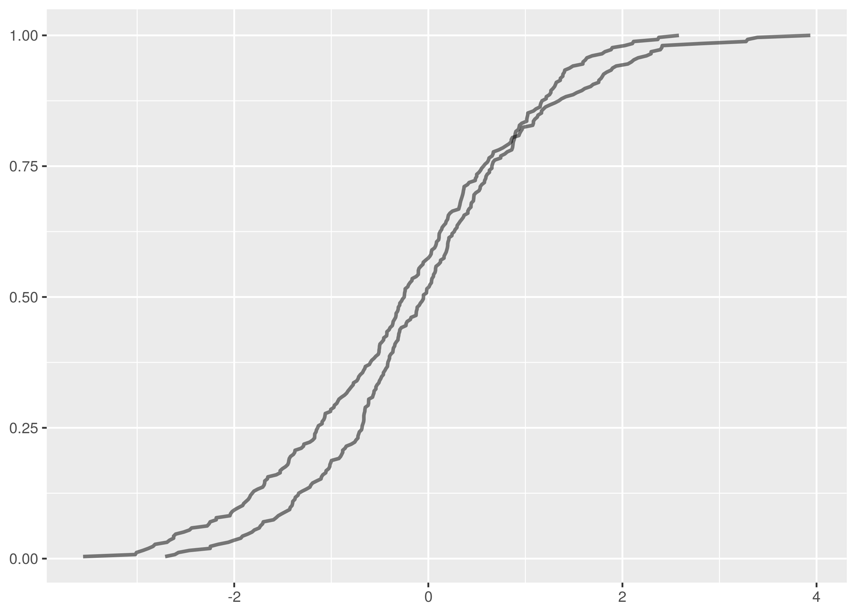
and  samples, the maximum vertical distance between the lines is at about -1.5 and 1.5.
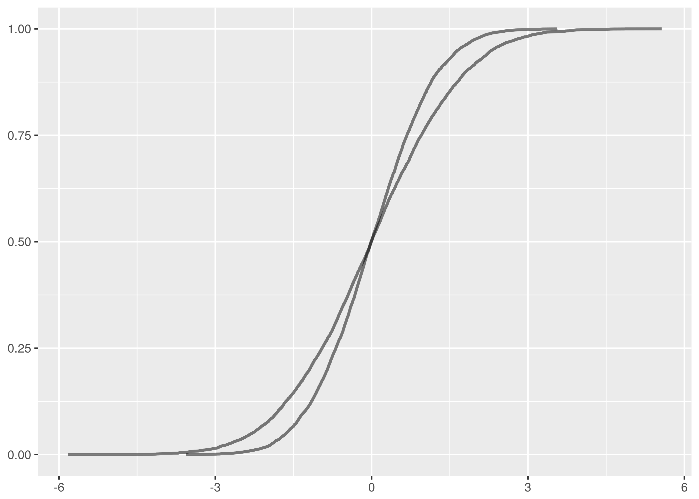
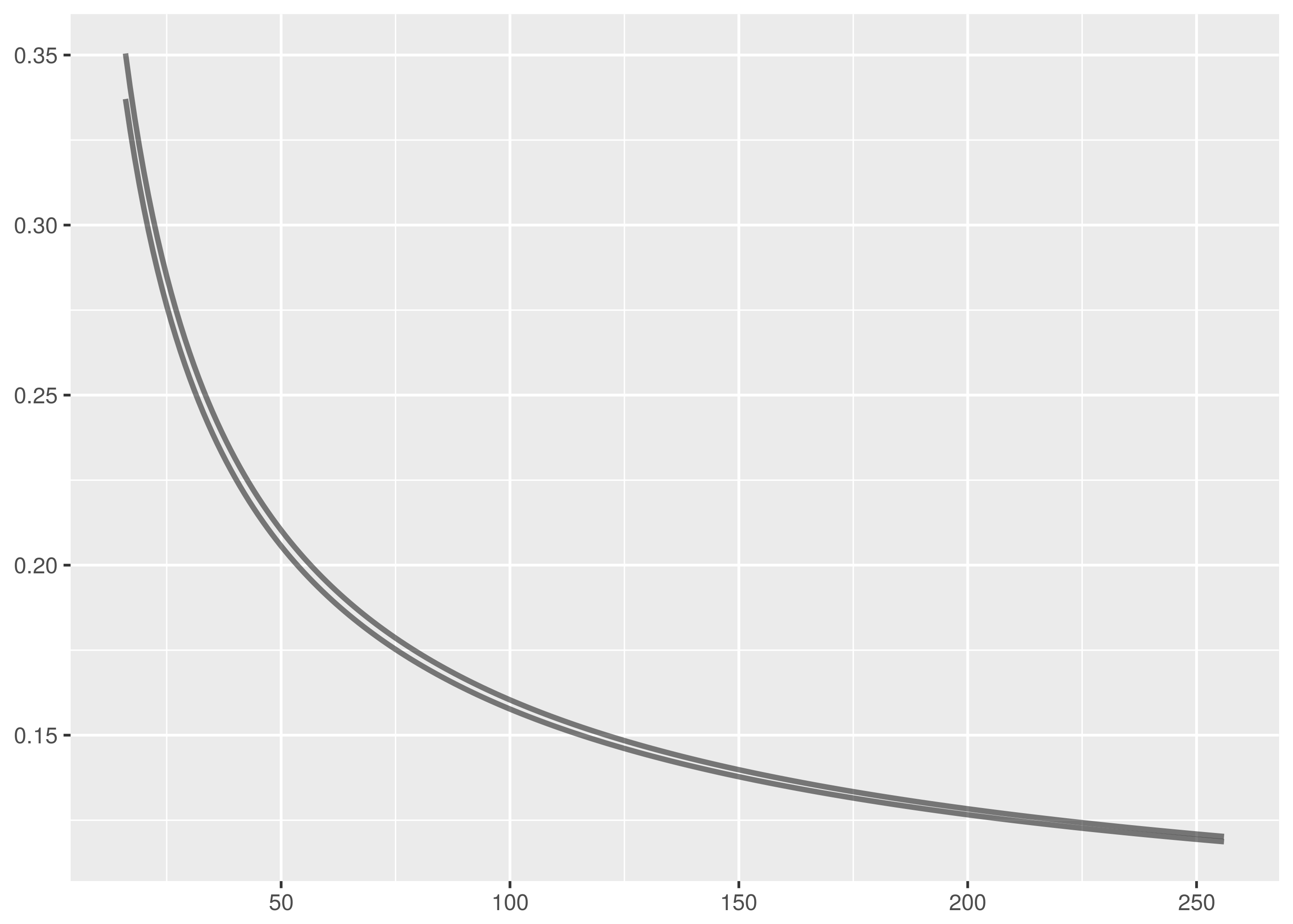
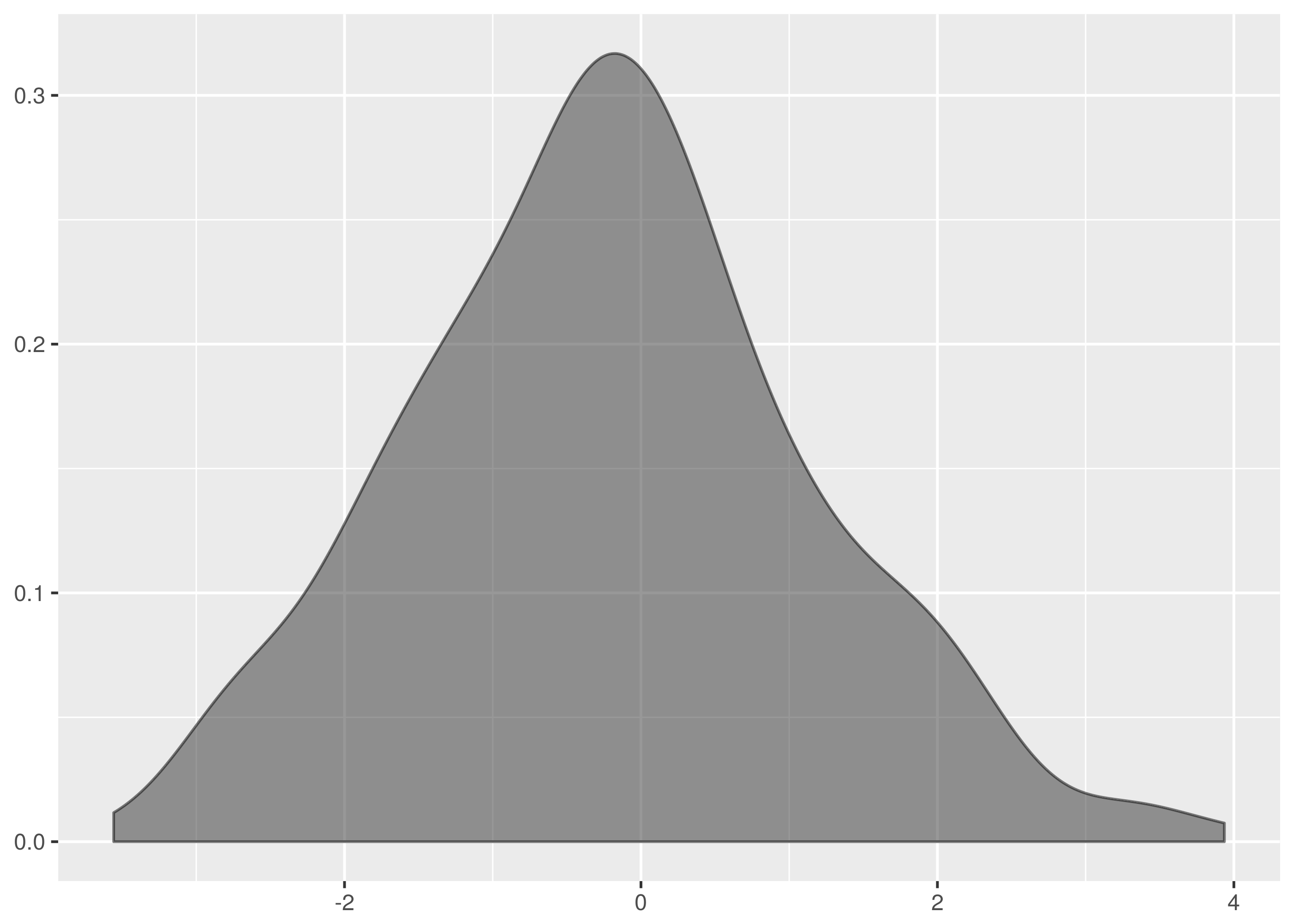
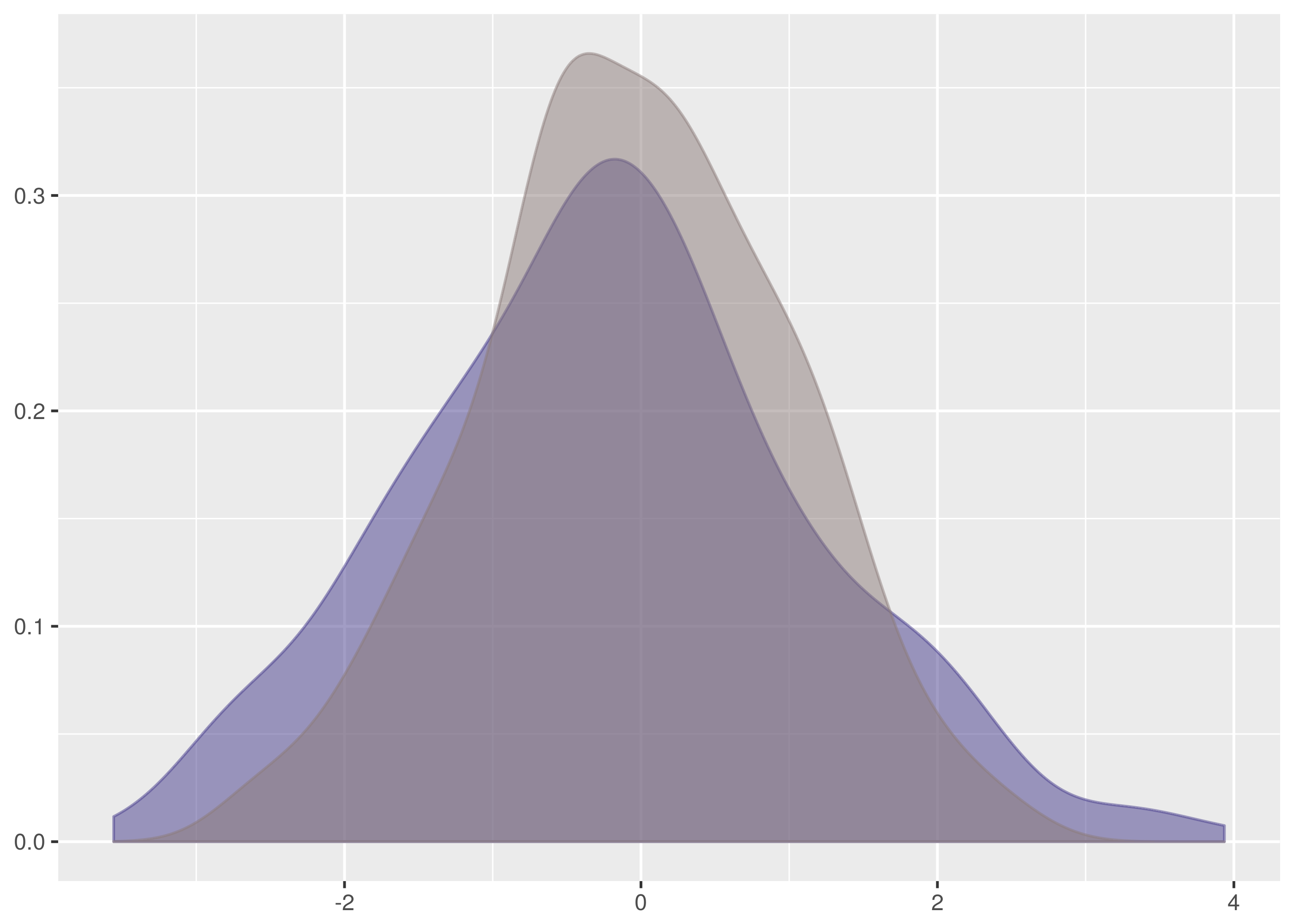
 . The maximum vertical distance occurs somewhere around zero and is quite large, maybe about 0.35 in size. This is significant evidence that the two samples are from different distributions.
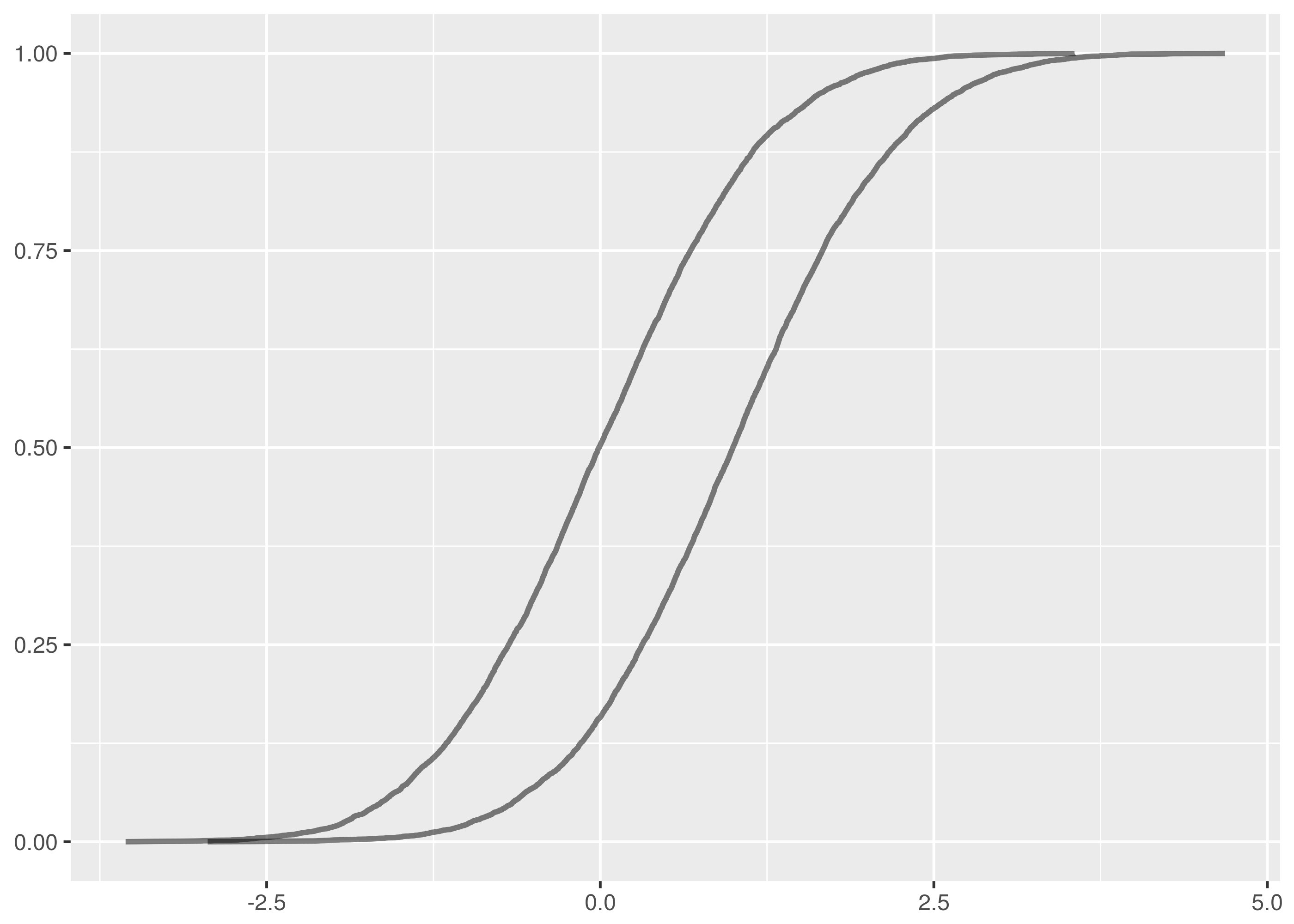
 are n independent and identically distributed observations of a continuous value. The empirical cumulative distribution function,
  , is:
, is:![F_n(x) = \frac{1}{n}\sum_{i=1}^n I_{(-\infty,x]}(X_i)](http://daithiocrualaoich.github.io/kolmogorov_smirnov/_images/math/fa8efad541845aeb3a36cade8cee92dd96075140.png)
 is the indicator function which is 1 if
  and 0 otherwise.
 is the number of samples observed that are less than or equal to
  , the Kolmogorov-Smirnov test statistic,
  , is the maximum absolute difference between
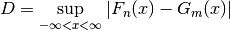
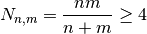
 for which
  .
.
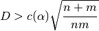
 .
.![P(D > \text{observed}) = Q_{KS}\Big(\Big[\sqrt{N_{n, m}} + 0.12 + 0.11/\sqrt{N_{n, m}}\Big] D\Big)](http://daithiocrualaoich.github.io/kolmogorov_smirnov/_images/math/650b24b8ef315acfdd6eeca0ab02d81cceed9db7.png)
 defined as:
 and drawing attention to the limitations of the floating point represention of irrational numbers.
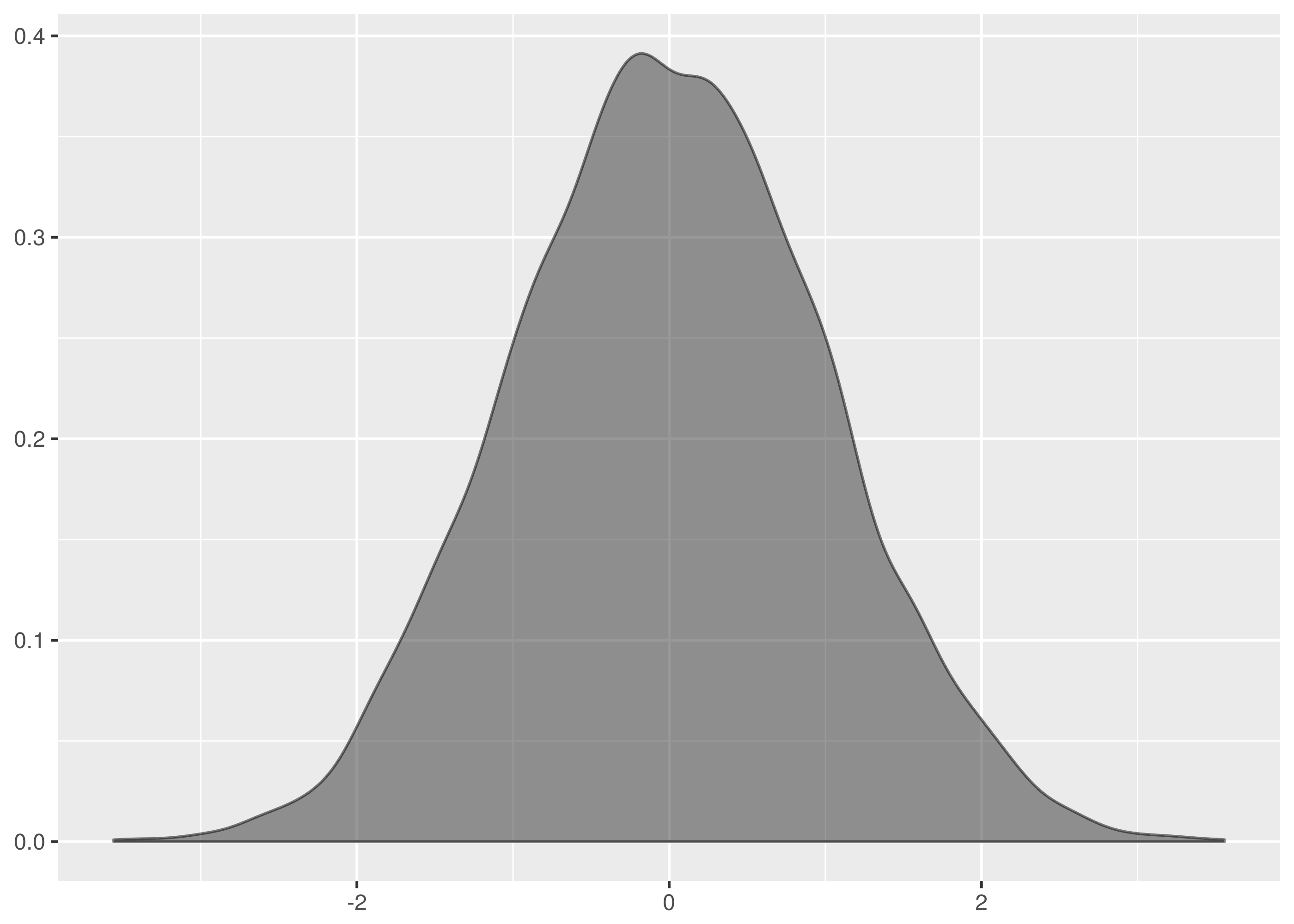
 ,
, ,
, ,
, .
. ,
,


 If an API allows hundreds of different connections concurrent access to the database, bad stuff will happen.
