A visit to a data and statistical technique useful to software engineers. We learn about some Rust too along the way.
The code and examples here are available on Github. The Rust library is on crates.io.
Kolmogorov-Smirnov Hypothesis Testing
The Kolmogorov-Smirnov test is a hypothesis test procedure for determining if two samples of data are from the same distribution. The test is non-parametric and entirely agnostic to what this distribution actually is. The fact that we never have to know the distribution the samples come from is incredibly useful, especially in software and operations where the distributions are hard to express and difficult to calculate with.
It is really surprising that such a useful test exists. This is an unkind Universe, we should be completely on our own.
The test description may look a bit hard in the outline below but skip ahead to the implementation because the Kolmogorov-Smirnov test is incredibly easy in practice.
The Kolmogorov-Smirnov test is covered in Numerical Recipes. There is a pdf available from the third edition of Numerical Recipes in C.
The Wikipedia article is a useful overview but light about proof details. If you are interested in why the test statistic has a distribution that is independent and useful for constructing the test then these MIT lecture notes give a sketch overview.
See this introductory talk by Toufic Boubez at Monitorama for an application of the Kolmogorov-Smirnov test to metrics and monitoring in software operations. The slides are available on slideshare.
The Test Statistic
The Kolmogorov-Smirnov test is constructed as a statistical hypothesis test. We determine a null hypothesis,  , that the two samples we are testing come from the same distribution. Then we search for evidence that this hypothesis should be rejected and express this in terms of a probability. If the likelihood of the samples being from different distributions exceeds a confidence level we demand the original hypothesis is rejected in favour of the hypothesis,
  , that the two samples are from different distributions.
To do this we devise a single number calculated from the samples, i.e. a statistic. The trick is to find a statistic which has a range of values that do not depend on things we do not know. Like the actual underlying distributions in this case.
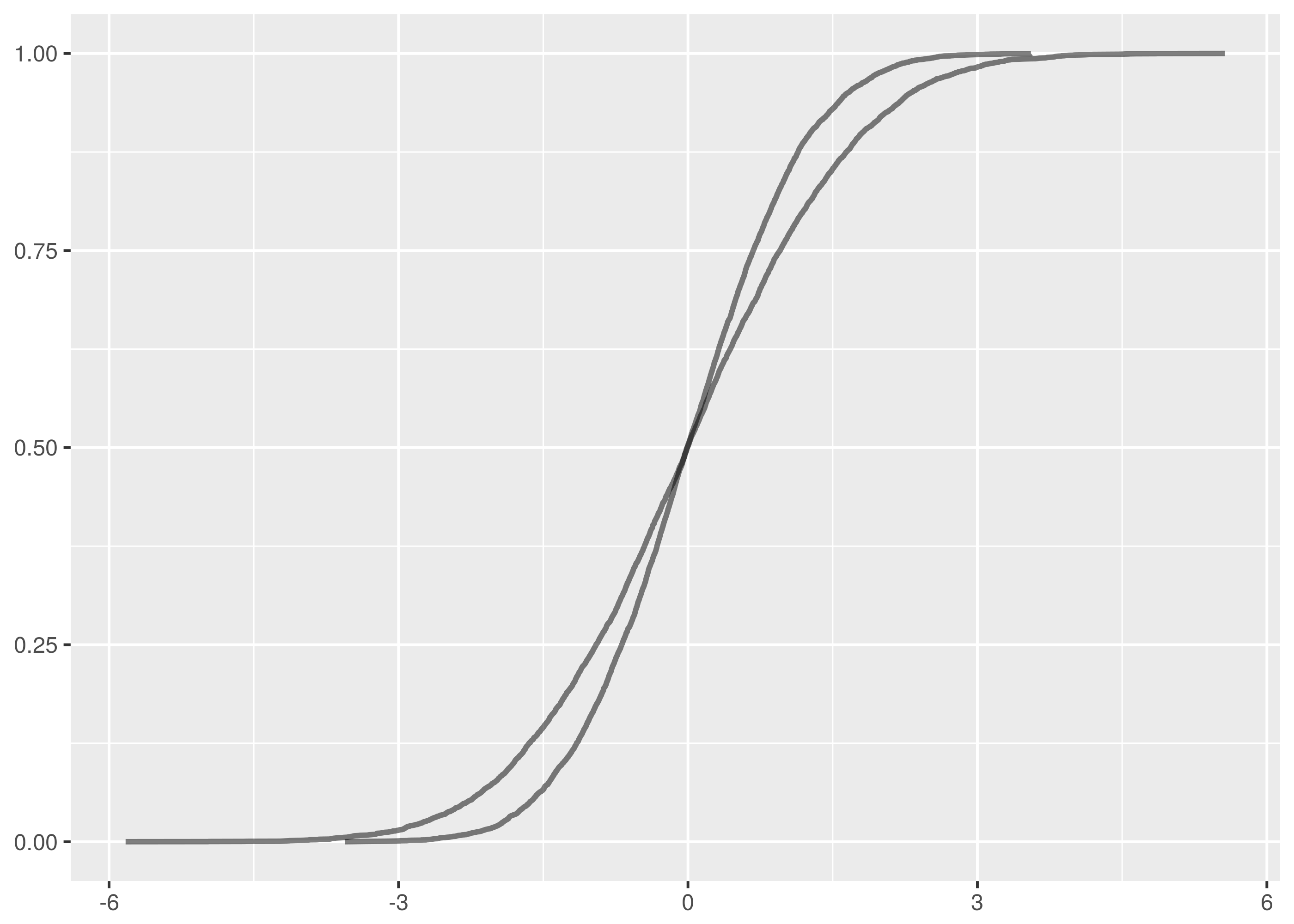
The test statistic in the Kolmogorov-Smirnov test is very easy, it is just the maximum vertical distance between the empirical cumulative distribution functions of the two samples. The empirical cumulative distribution of a sample is the proportion of the sample values that are less than or equal to a given value.
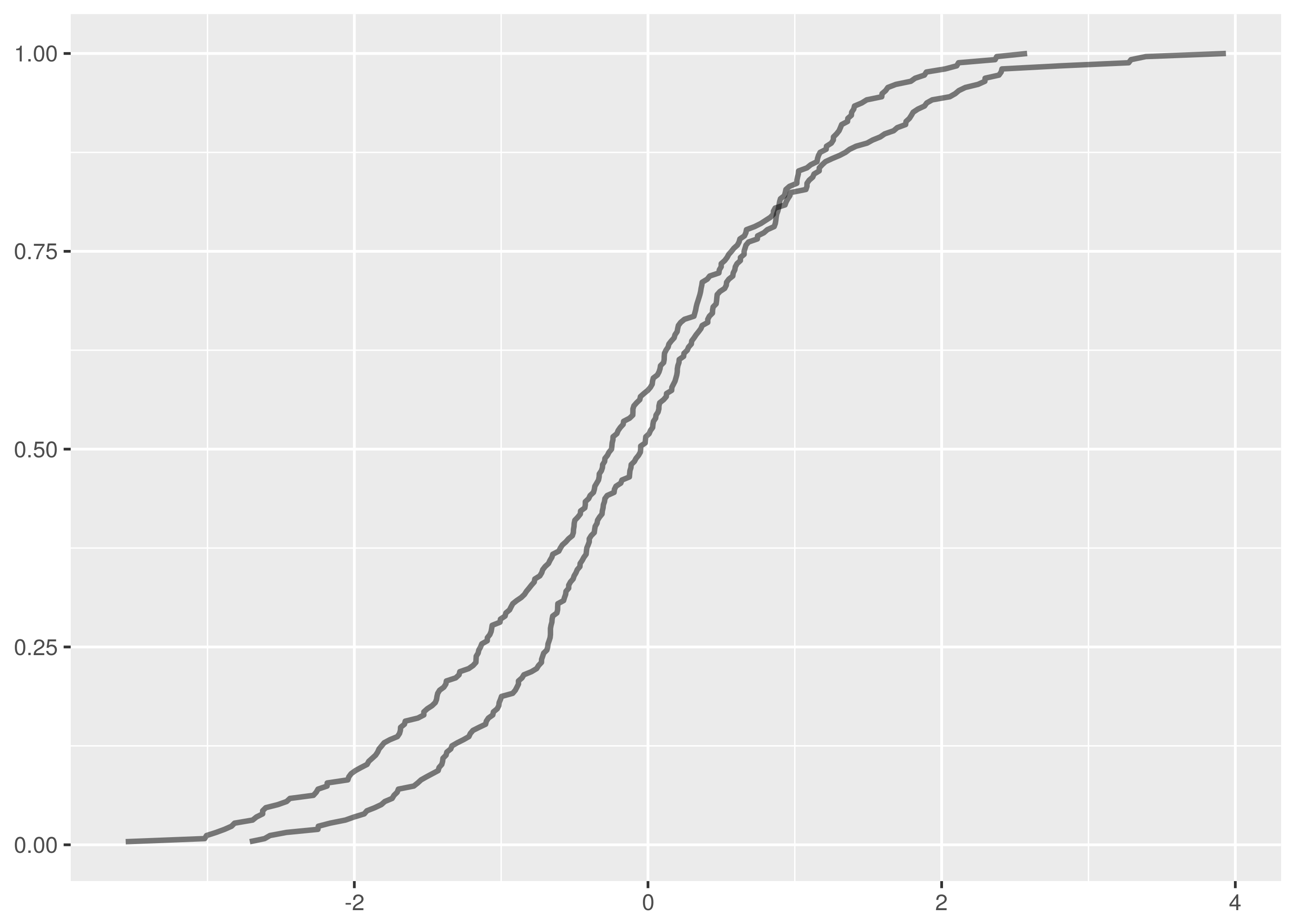
For instance, in this plot of the empirical cumulative distribution functions of normally distributed data,  and
and  samples, the maximum vertical distance between the lines is at about -1.5 and 1.5.
The vertical distance is a lot clearer for an sample against  . The maximum vertical distance occurs somewhere around zero and is quite large, maybe about 0.35 in size. This is significant evidence that the two samples are from different distributions.
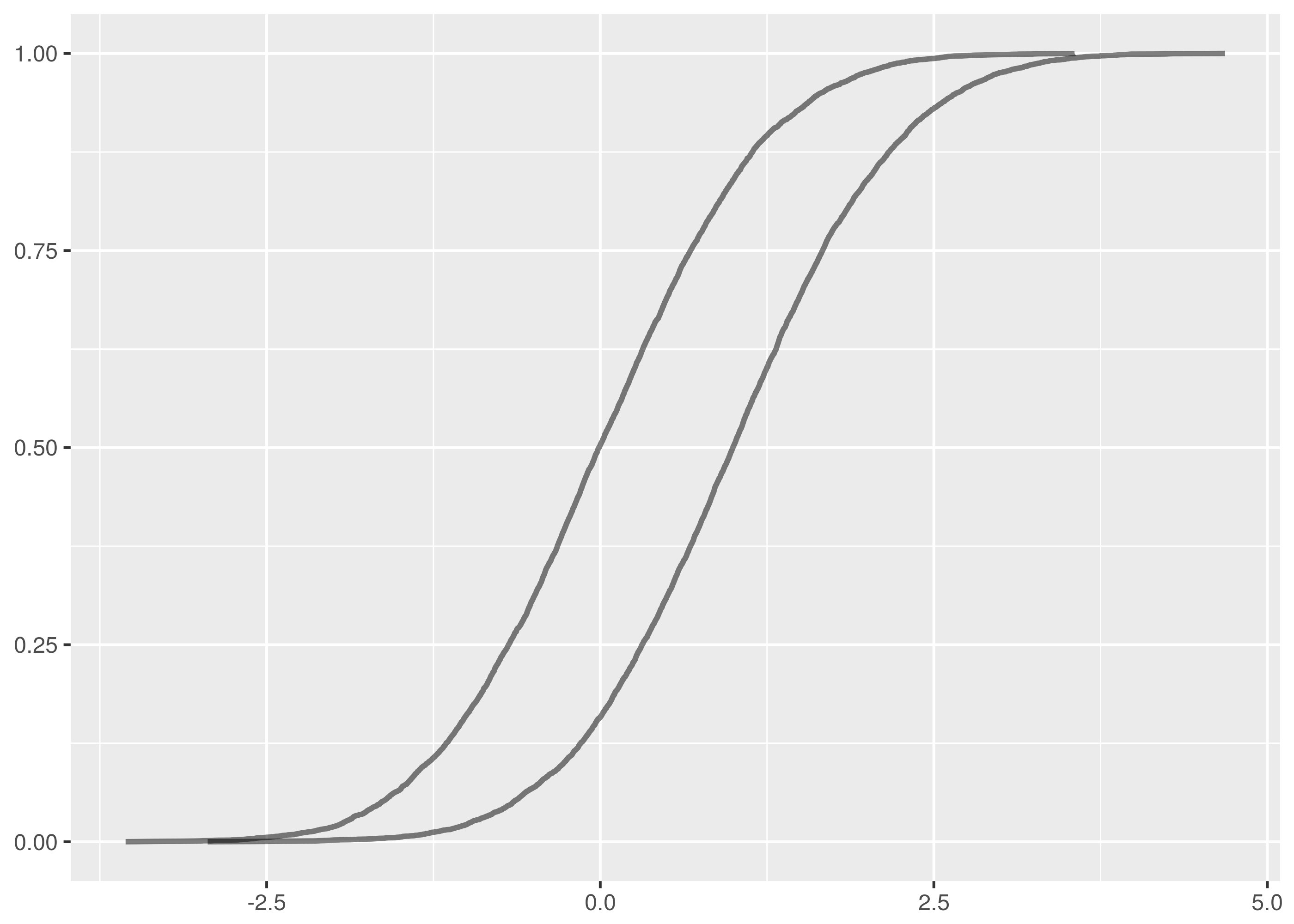
As an aside, these examples demonstrate an important note about the application of the Kolomogorov-Smirnov test. It is much better at detecting distributional differences when the sample medians are far apart than it is at detecting when the tails are different but the main mass of the distributions is around the same values.
So, more formally, suppose  are n independent and identically distributed observations of a continuous value. The empirical cumulative distribution function,
  , is:
, is:
![F_n(x) = \frac{1}{n}\sum_{i=1}^n I_{(-\infty,x]}(X_i)](http://daithiocrualaoich.github.io/kolmogorov_smirnov/_images/math/fa8efad541845aeb3a36cade8cee92dd96075140.png)
Where  is the indicator function which is 1 if is less than or equal to
  and 0 otherwise.
This just says that  is the number of samples observed that are less than or equal to divided by the total number of samples. But it says it in a complicated way so we can feel clever about ourselves.
The empirical cumulative distribution function is an unbiased estimator for the underlying cumulative distribution function, incidentally.
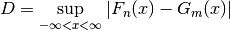
For two samples having empirical cumulative distribution functions and  , the Kolmogorov-Smirnov test statistic,
  , is the maximum absolute difference between and for the same , i.e. the largest vertical distance between the plots in the graph.
The Glivenko–Cantelli theorem says if the is made from samples from the same distribution as then this statistic “almost surely converges to zero in the limit when n goes to infinity.” This is an extremely technical statement that we are simply going to ignore.
Two Sample Test
Surprisingly, the distribution of can be approximated well in the case that the samples are drawn from the same distribution. This means we can build a statistic test that rejects this null hypothesis for a given confidence level if exceeds an easily calculable value.
Tables of critical values are available, for instance the SOEST tables describe a test implementation for samples of more than twelve where we reject the null hypothesis, i.e. decide that the samples are from different distributions, if:
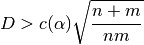
Where n and m are the sample sizes. A 95% confidence level corresponds to  for which
  .
.
Alternatively, Numerical Recipes describes a direct calculation that works well for:
i.e. for samples of more than seven since  .
.
Numerical Recipes continues by claiming the probability that the test statistic is greater than the value observed is approximately:
![P(D > \text{observed}) = Q_{KS}\Big(\Big[\sqrt{N_{n, m}} + 0.12 + 0.11/\sqrt{N_{n, m}}\Big] D\Big)](http://daithiocrualaoich.github.io/kolmogorov_smirnov/_images/math/650b24b8ef315acfdd6eeca0ab02d81cceed9db7.png)
With  defined as:
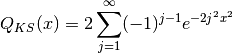
This can be computed by summing terms until a convergence criteria is achieved. The implementation in Numerical Recipes gives this a hundred terms to converge before failing.
The difference between the two approximations is marginal. The Numerical Recipes approach produces slightly smaller critical values for rejecting the null hypothesis as can be seen in the following plot of critical values for the 95% confidence level where one of the samples has size 256. The x axis varies over the other sample size, the y axis being the critical value.
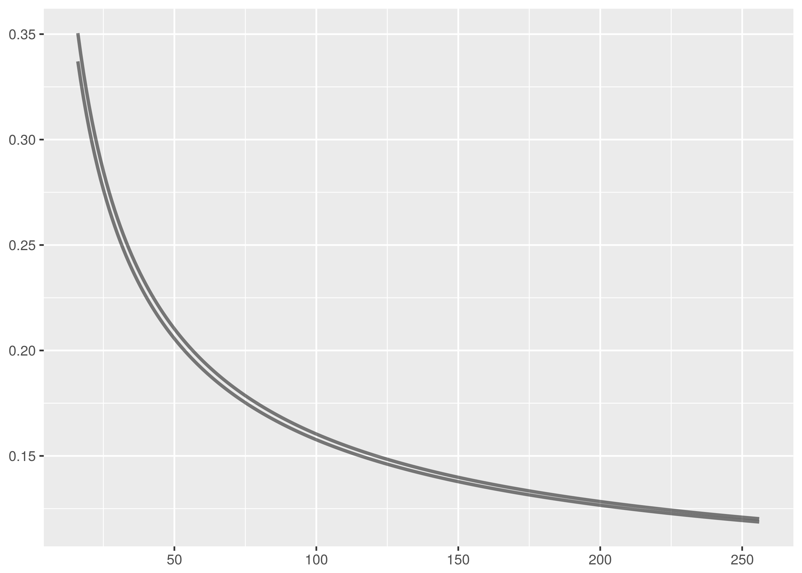
The SOEST tables are an excellent simplifying approximation.
Discussion
A straightforward implementation of this test can be found in the Github repository. Calculating the test statistic using the empirical cumulative distribution functions is probably as complicated as it gets for this. There are two versions of the test statistic calculation in the code, the simpler version being used to probabilistically verify the more efficient implementation.
Non-parametricity and generality are the great advantages of the Kolomogorov-Smirnov test but these are balanced by drawbacks in ability to establish sufficient evidence to reject the null hypothesis.
In particular, the Kolmogorov-Smirnov test is weak in cases when the sample empirical cumulative distribution functions do not deviate strongly even though the samples are from different distributions. For instance, the Kolomogorov-Smirnov test is most sensitive to discrepency near the median of the samples because this is where differences in the graph are most likely to be large. It is less strong near the tails because the cumulative distribution functions will both be near 0 or 1 and the difference between them less pronounced. Location and shape related scenarios that constrain the test statistic reduce the ability of the Kolmogorov-Smirnov test to correctly reject the null hypothesis.
The Chi-squared test is also used for testing whether samples are from the same distribution but this is done with a binning discretization of the data. The Kolomogorov-Smirnov test does not require this.
A Field Manual for Rust
Rust is a Mozilla sponsored project to create a safe, fast systems language. There is an entire free O’Reilly book on why create this new language but the reasons include:
- Robust memory management. It is impossible to deference null or dangling pointers in Rust.
- Improved security, reducing the incidence of flaws like buffer overflow exploits.
- A light runtime with no garbage collection and overhead means Rust is ideal to embed in other languages and platforms like Ruby, Python, and Node.
- Rust has many modern language features unavailable in other systems languages.
Rust is a serious language, capable of very serious projects. The current flagship Rust project, for instance, is Servo, a browser engine under open source development with contributions from Mozilla and Samsung.
The best introduction to Rust is the Rust Book. Newcomers should also read Steve Klabnik’s alternative introdution to Rust for the upfront no-nonsense dive into memory ownership, the crux concept for Rust beginners.
Those in a hurry can quickstart with these slide decks by:
Two must-read learning resources are 24 Days of Rust, a charming tour around the libraries and world of Rust, and ArcadeRS, a tutorial in Rust about writing video games.
And finally, if Servo has you interested in writing a browser engine in Rust, then Let’s build a browser engine! is the series for you. It walks through creating a simple HTML rendering engine in Rust.
Moral Support for Learning the Memory Rules
The Road to Rust is not royal, there is no pretending otherwise. The Rust memory rules about lifetime, ownership, and borrowing are especially hard to learn.
It probably doesn’t much feel like it but Rust is really trying to help us with these rules. And to be fair to Rust, it hasn’t segfaulted me so far.
But that is no comfort when the compiler won’t build your code and you can’t figure out why. The best advice is probably to read as much about the Rust memory rules as you can and to keep reading about them over and over until they start to make some sense. Don’t worry, everybody finds it difficult at first.
Although adherence to the rules provides the compiler with invariant guarantees that can be used to construct proofs of memory safety, the rationale for these rules is largely unimportant. What is necessary is to find a way to work with them so your programs compile.
Remember too that learning to manage memory safely in C/C++ is much harder than learning Rust and there is no compiler checking up on you in C/C++ to make sure your memory management is correct.
Keep at it. It takes a long time but it does become clearer!
Niche Observations
This section is a scattering of Rust arcana that caught my attention. Nothing here that doesn’t interest you is worth troubling too much with and you should skip on past.
Travis CI has excellent support for building Rust projects, including with the beta and nightly versions. It is simple to set up by configuring a travis.yml according to the Travis Rust documentation. See the Travis CI build for this project for an example.
Rust has a formatter in rustfmt and a lint in rust-clippy. The formatter is a simple install using cargoinstall and provides a binary command. The lint requires more integration into your project, and currently also needs the nightly version of Rust for plugin support. Both projects are great for helping Rust newcomers.
Foreign Function Interface is an area where Rust excels. The absence of a large runtime means Rust is great for embedding in other languages and it has a wide range as a C replacement in writing modules for Python, Ruby, Node, etc. The Rust Book introduction demonstrates how easy it is call Rust from other languages. Day 23 of Rust and the Rust FFI Omnibus are additional resources for Rust FFI.
Rust is being used experimentally for embedded development. Zinc is work on building a realtime ARM operating system using Rust primarily, and the following are posts about building software for embedded devices directly using Rust.
Relatedly, Rust on Raspberry Pi is a guide to cross-compiling Rust code for the Raspberry Pi.
Rust treats the code snippets in your project documentation as tests and makes a point of compiling them. This helps keep documentation in sync with code but it is a shock the first time you get a compiler error for a documentation code snippet and it takes you ages to realise what is happening.
Kolmogorov-Smirnov Library
The Kolmogorov-Smirnov test implementation is available as a Cargo crate, so it is simple to incorporate into your programs. Add the dependency to your Cargo.toml file.
[dependencies]kolmogorov_smirnov="1.0.1"Then to use the test, call the kolmogorov_smirnov::test function with the two samples to compare and the desired confidence level.
externcratekolmogorov_smirnovasks;letxs=vec!(0,1,2,3,4,5,6,7,8,9,10,11,12);letys=vec!(12,11,10,9,8,7,6,5,4,3,2,1,0);letconfidence=0.95;letresult=ks::test(&xs,&ys,confidence);if!result.is_rejected{// Woot! Samples are from the same distribution with 0.95 confidence.}The Kolmogorov-Smirnov test as implemented works for any data with a Clone and an Ord trait implementation in Rust. So it is possible, but pretty useless, to test samples of characters, strings and lists. In truth, the Kolmorogov-Smirnov test requires the samples to be taken from a continuous distribution, so discrete data like characters and strings are cute to consider but invalid test data.
Still being strict, this test condition also does not hold for integer data unless some hands are waved about the integer data being embedded into real numbers and a distribution cooked up from the probability weights. We make some compromises and allowances.
If you have floating point or integer data to test, you can use the included test runner binaries, ks_f64 and ks_i32. These operate on single-column headerless data files and test two commandline argument filenames against each other at 95% confidence.
$ cargo run -q --bin ks_f64 dat/normal_0_1.tsv dat/normal_0_1.1.tsv
Samples are from the same distribution.
test statistic = 0.0399169921875
critical value = 0.08550809323787689
reject probability = 0.18365715210599798

$ cargo run -q --bin ks_f64 dat/normal_0_1.tsv dat/normal_1_1.1.tsv
Samples are from different distribution.
test statistic = 0.361572265625
critical value = 0.08550809323787689
reject probability = 1
Testing floating point numbers is a headache because Rust floating point types (correctly) do not implement the Ord trait, only the PartialOrd trait. This is because things like NaN are not comparable and the order cannot be total over all values in the datatype.
The test runner for floating point types is implemented using a wrapper type that implements a total order, crashing on unorderable elements. This suffices in practice since the unorderable elements will break the test anyway.
The implementation uses the Numerical Recipes approximation for rejection probabilities rather than the almost as accurate SOEST table approximation for critical values. This allows the additional reporting of the reject probability which isn’t available using the SOEST approach.
Datasets
Statistical tests are more fun if you have datasets to run them over.
N(0,1)
Because it is traditional and because it is easy and flexible, start with some normally distributed data.
Rust can generate normal data using the rand::distributions module. If mean and variance are f64 values representing the mean and variance of the desired normal deviate, then the following code generates the deviate. Note that the Normal::new call requires the mean and standard deviation as parameters, so it is necessary to take the square root of the variance to provide the standard deviation value.
externcraterand;userand::distributions::{Normal,IndependentSample};letmean:f64=...letvariance:f64=...letmutrng=rand::thread_rng();letnormal=Normal::new(mean,variance.sqrt());letx=normal.ind_sample(&mutrng);The kolmogorov_smirnov library includes a binary for generating sequences of independently distributed Normal deviates. It has the following usage.
cargo run --bin normal <num_deviates> <mean> <variance>
The -q option is useful too for suppressing cargo build messages in the output.
Sequences from , , and are included in the Github repository. is included mainly just to troll, calculating  and drawing attention to the limitations of the floating point represention of irrational numbers.
cargo run -q --bin normal 819201> normal_0_1.tsv
cargo run -q --bin normal 819202> normal_0_2.tsv
cargo run -q --bin normal 819211> normal_1_1.tsv
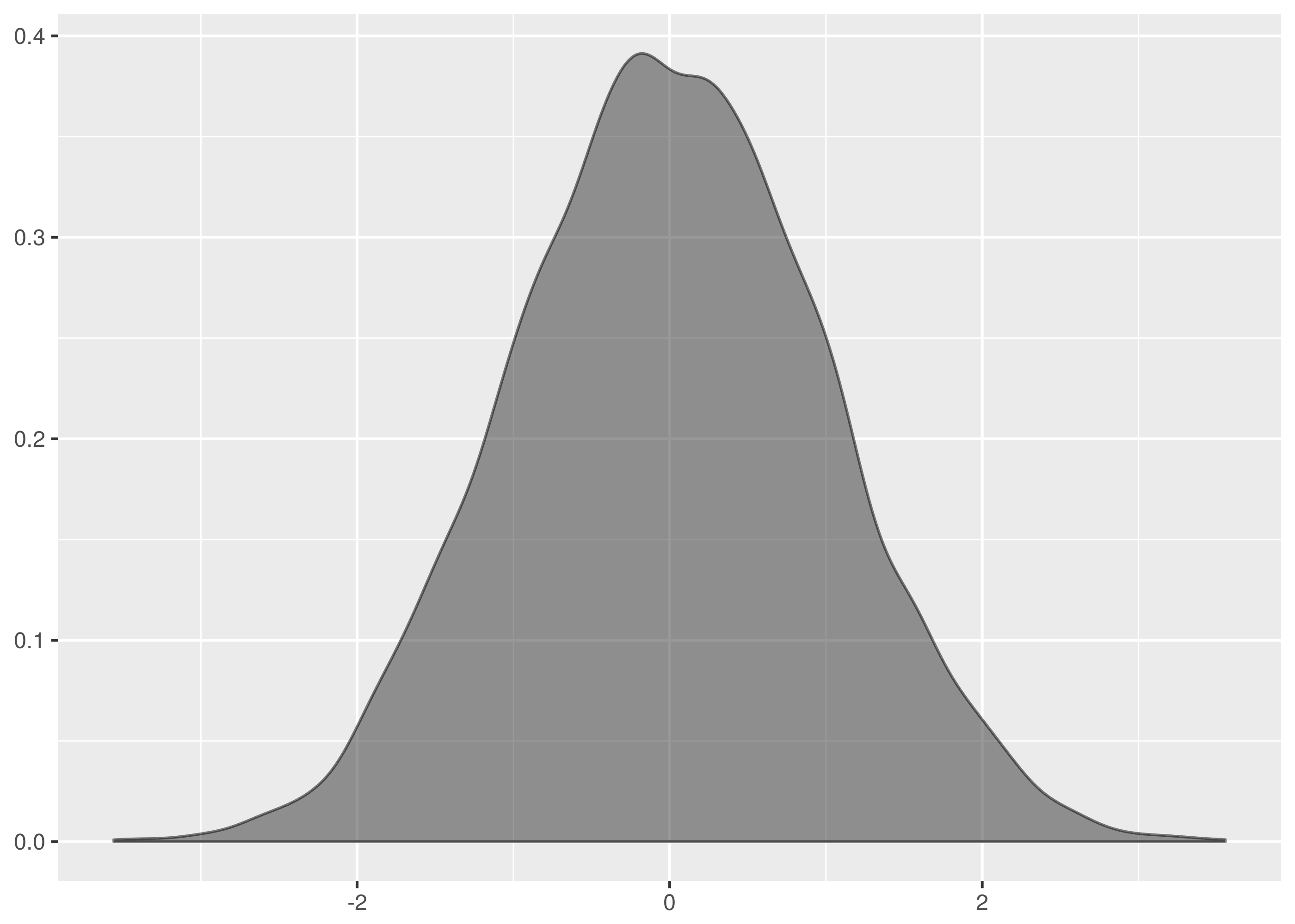
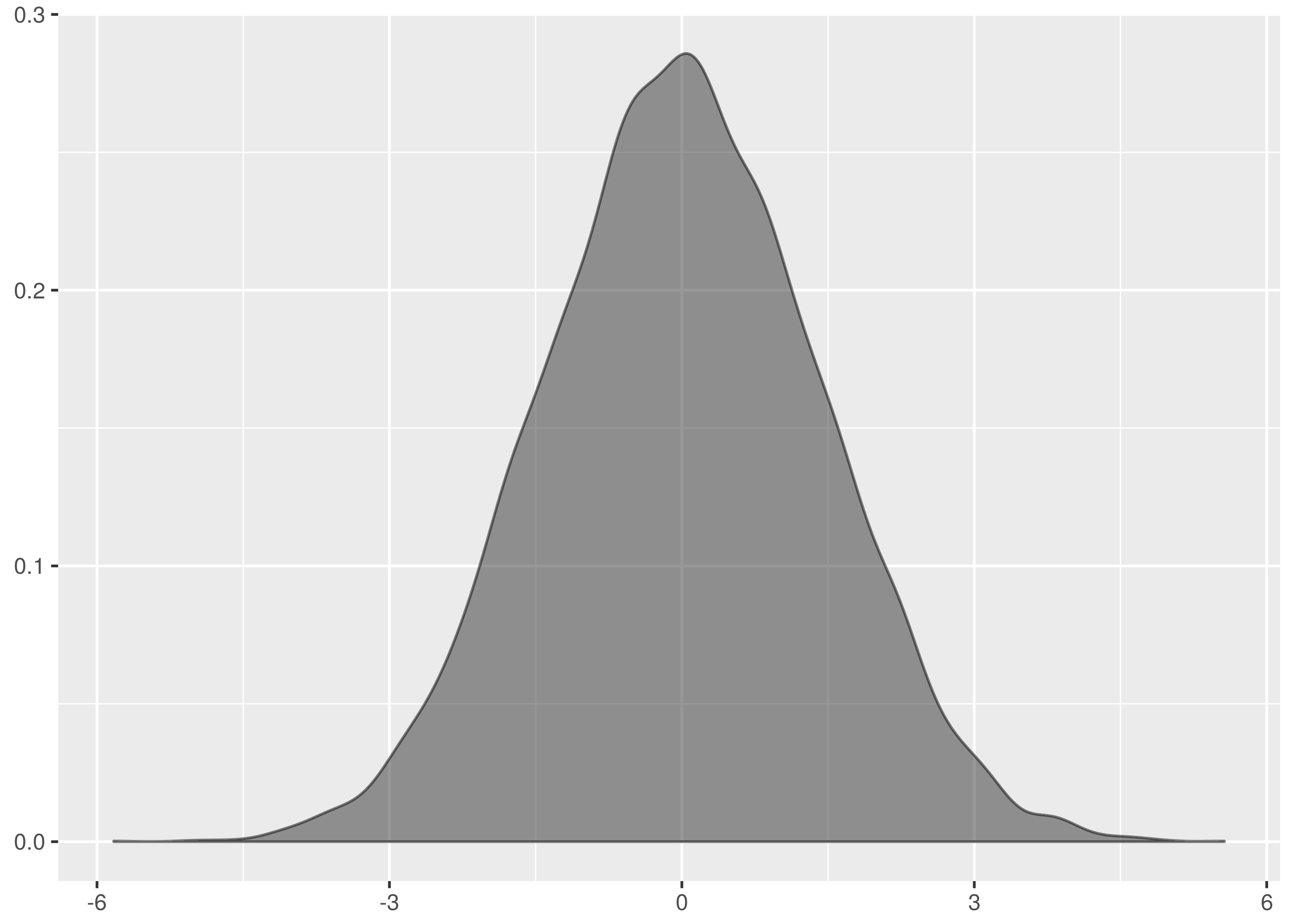
These are not the most beautiful of Normal curves, but you must take what you get. The data is lumpy and not single peaked.
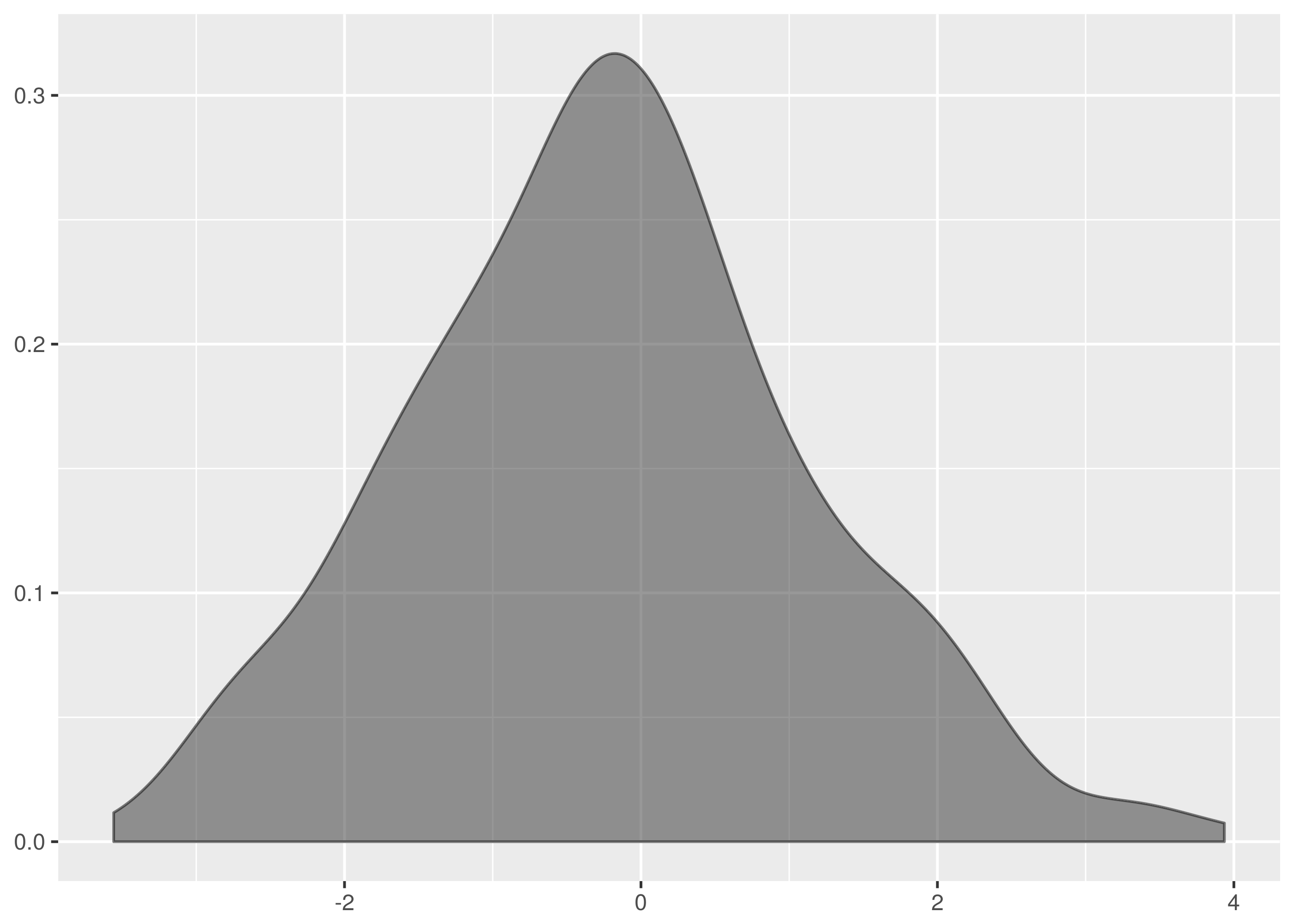
is similar, though less of a disaster near the mean.
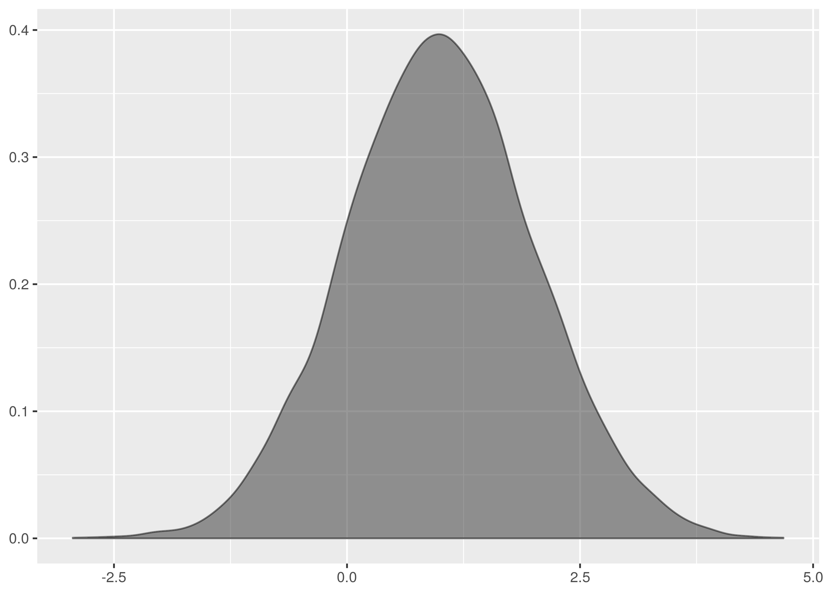
by contrast looks suprisingly like the normal data diagrams in textbooks.
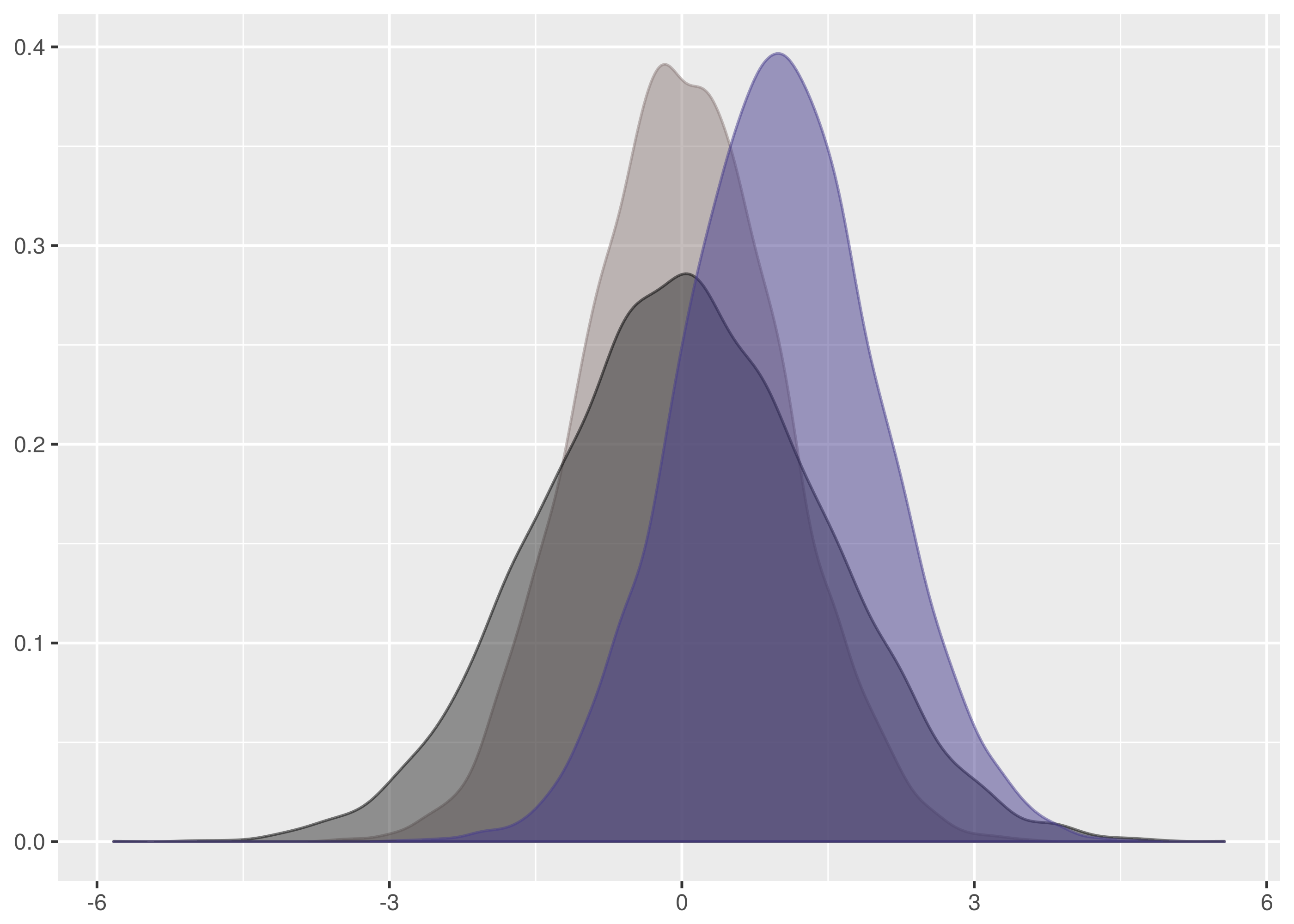
The following is a plot of all three datasets to illustrate the relative widths, heights and supports.
Results
The Kolmogorov-Smirnov test is successful at establishing the datasets are all from the same distribution in all combinations of the test.
$ cargo run -q --bin ks_f64 dat/normal_0_1.tsv dat/normal_0_1.1.tsv
Samples are from the same distribution.
test statistic = 0.0399169921875
critical value = 0.08550809323787689
reject probability = 0.18365715210599798

$ cargo run -q --bin ks_f64 dat/normal_0_1.tsv dat/normal_0_1.2.tsv
Samples are from the same distribution.
test statistic = 0.0595703125
critical value = 0.08550809323787689
reject probability = 0.6677483327196572

...
Save yourself the trouble in reproduction by running this instead:
for I in dat/normal_0_1.*
dofor J in dat/normal_0_1.*
    doif[["$I"< "$J"]]thenecho$I$J
            cargo run -q --bin ks_f64 $I$Jecho            echofidonedone
The datasets also correctly accept the null hypothesis in all combinations of dataset inputs when tested against each other.
However, successfully passes for all combinations but that between dat/normal_0_2.tsv and dat/normal_0_2.1.tsv where it fails as a false negative.
$ cargo run -q --bin ks_f64 dat/normal_0_2.1.tsv dat/normal_0_2.tsv
Samples are from different distributions.
test statistic = 0.102783203125
critical value = 0.08550809323787689
reject probability = 0.9903113063475989
This failure is a demonstration of how the Kolmogorov-Smirnov test is sensitive to location because here the mean of the dat/normal_0_2.1.tsv is shifted quite far from the origin.
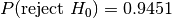
This is the density.
And superimposed with the density from dat/normal_0_2.tsv.
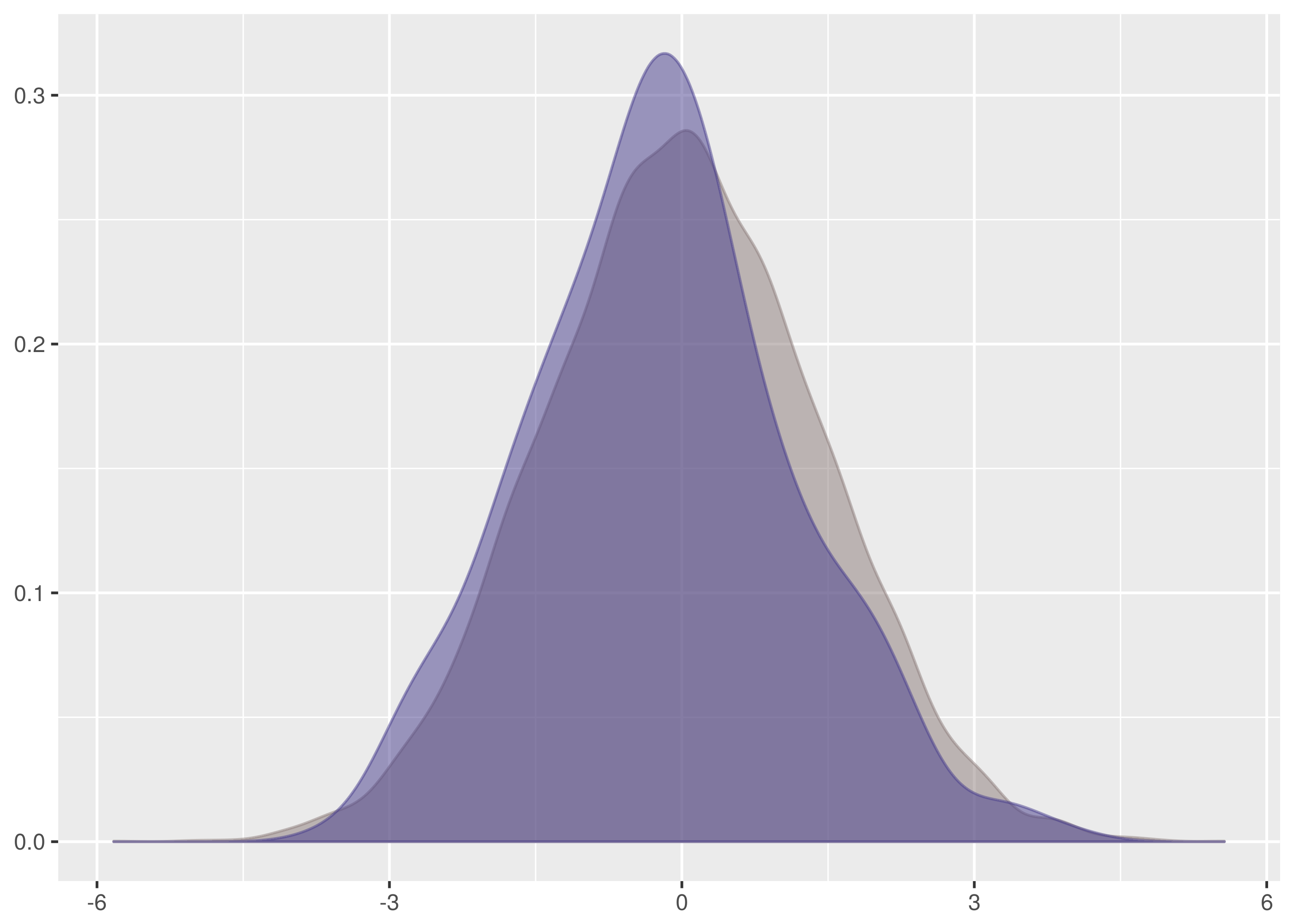
The data for dat/normal_0_2.1.tsv is the taller density in this graph. Notice, in particular, that the mean is shifted left a lot in comparison with dat/normal_0_2.tsv. See also the chunks of non-overlapping weight on the left and right hand slopes.
The difference in means is confirmed by calculation. The dataset for dat/normal_0_2.tsv has mean 0.001973723, whereas the dataset for dat/normal_0_2.1.tsv has mean -0.2145779. By comparison, the other datasets tests have means -0.1308625, -0.08537648, and -0.01374325.
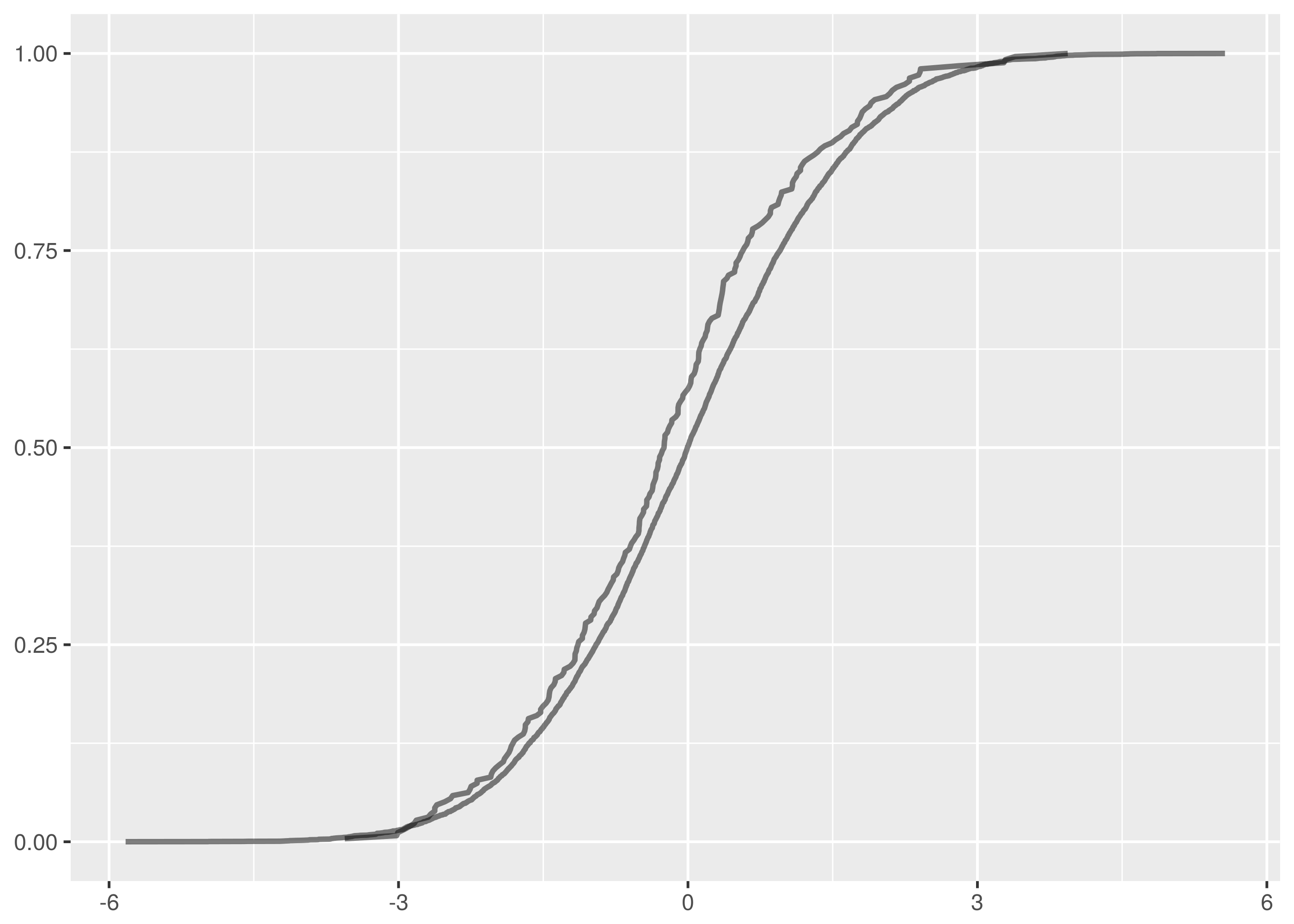
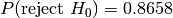
Looking at the empirical cumulative density functions of the false negative comparison, we see a significant gap between the curves starting near 0.
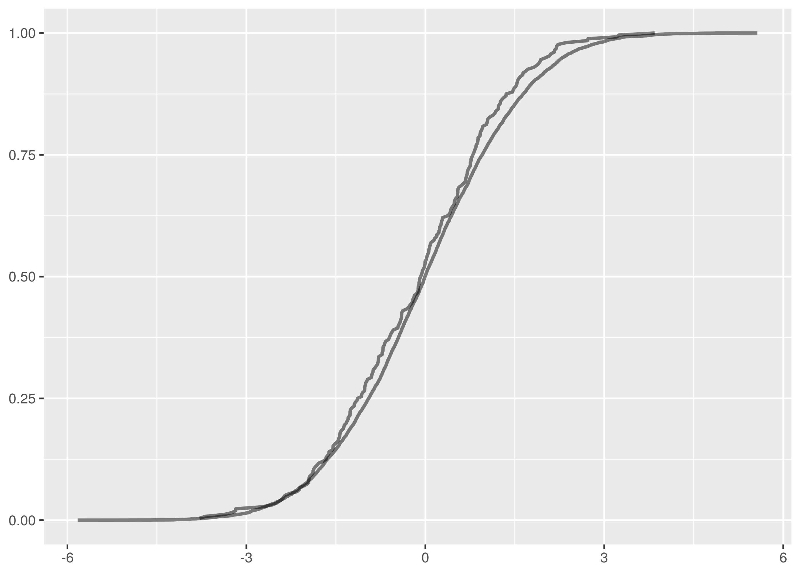
For comparison, here are the overlaid empirical cumulative density functions for the other tests.
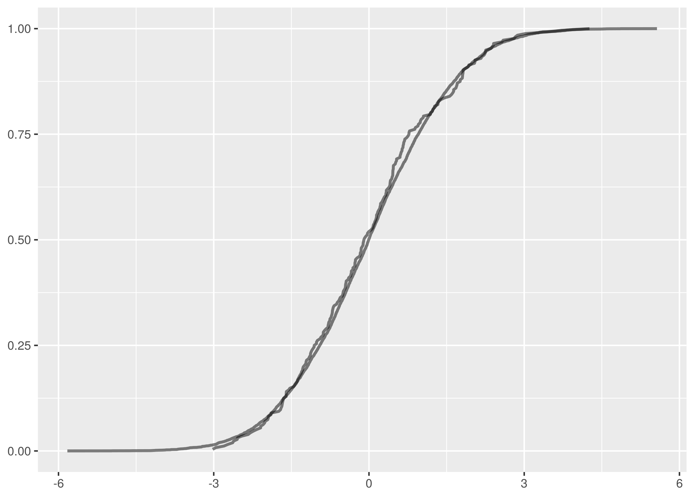
One false negative in thirty unique test pairs at 95% confidence is on the successful side of expectations.
Turning instead to tests that should be expected to fail, the following block runs comparisons between datasets from different distributions.
for I in dat/normal_0_1.*
dofor J in dat/normal_0_2.*
    doecho$I$J
        cargo run -q --bin ks_f64 $I$Jecho        echodonedone
The against and against tests correctly reject the null hypothesis in every variation. These tests are easy failures because they are large location changes, illustrating again how the Kolmogorov-Smirnov test is sensitive to changes in centrally located weight.
However, there are ten false positives in the comparisons between datasets from and .
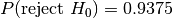
dat/normal_0_1.2.tsv is reported incorrectly as being from the same distribution as the following datasets.
dat/normal_0_2.tsvat![P(\text{reject } H_0) = 0.9375]() ,
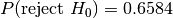
,dat/normal_0_2.2.tsvat![P(\text{reject } H_0) = 0.6584]() ,
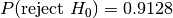
,dat/normal_0_2.3.tsvat![P(\text{reject } H_0) = 0.9128]() ,
,dat/normal_0_2.4.tsvat![P(\text{reject } H_0) = 0.8658]() .
.
 ,
, ,
, ,
, .
.Similarly, dat/normal_0_1.3.tsv is a false positive against:
dat/normal_0_2.3.tsvat![P(\text{reject } H_0) = 0.9128]() ,
,dat/normal_0_2.4.tsvat![P(\text{reject } H_0) = 0.8658]() .
.
And dat/normal_0_1.4.tsv is a false positive against:
dat/normal_0_2.1.tsvat![P(\text{reject } H_0) = 0.9451]() ,
,dat/normal_0_2.2.tsvat![P(\text{reject } H_0) = 0.9451]() ,
,dat/normal_0_2.3.tsvat![P(\text{reject } H_0) = 0.9128]() ,
,dat/normal_0_2.4.tsvat![P(\text{reject } H_0) = 0.9128]() .
.
 ,
,Note that many of these false positives have rejection probabilities that are high but fall short of the 95% confidence level required. The null hypothesis is that the distributions are the same and it is this that must be challenged at the 95% level.
Let’s examine the test where the rejection probability is lowest, that between dat/normal_0_1.2.tsv and dat/normal_0_2.2.tsv.
$ cargo run -q --bin ks_f64 dat/normal_0_1.2.tsv dat/normal_0_2.2.tsv
Samples are from the same distribution.
test statistic = 0.08203125
critical value = 0.11867932230234146
reject probability = 0.6584658436106378
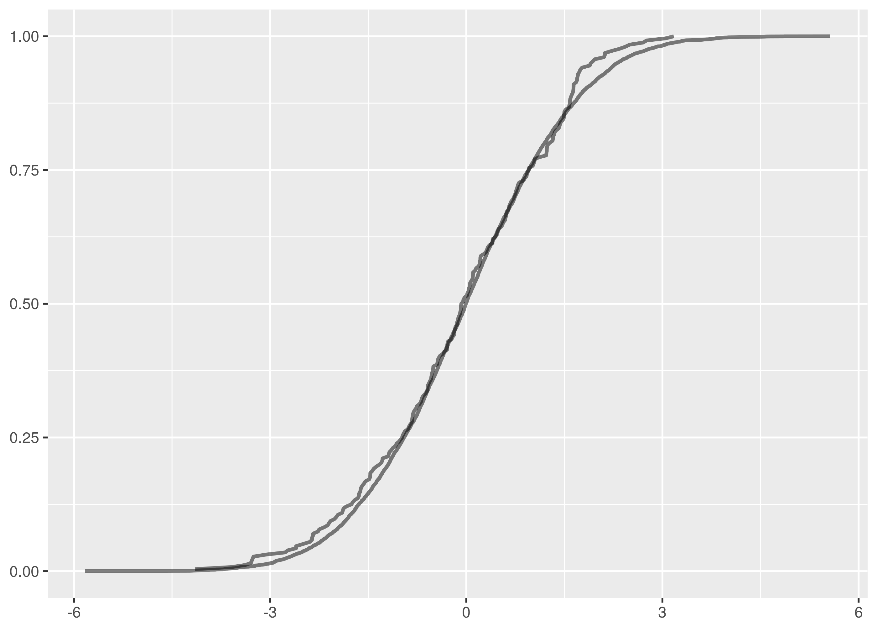
The overlaid density and empirical cumulative density functions show strong difference.

The problem, however, is a lack of samples combined with the weakness of the Kolmogorov-Smirnov test in detecting differences in spread at the tails. Both of these datasets have 256 samples and the critical value for 95% confidence is 0.1186. This is a large difference to demonstrate at the edges of the empirical cumulative distribution functions and in the case of this test the test statistic is a comfortable 0.082.
There is insufficient evidence to reject the null hypothesis.
Let’s also examine the false positive test where the rejection probability is tied highest, between dat/normal_0_1.4.tsv and dat/normal_0_2.1.tsv.
$ cargo run -q --bin ks_f64 dat/normal_0_1.4.tsv dat/normal_0_2.1.tsv
Samples are from the same distribution.
test statistic = 0.1171875
critical value = 0.11867932230234146
reject probability = 0.9451734528250557
This is just incredibly borderline. There is very strong difference on the left side but it falls fractionally short of the required confidence level. Note how this also illustrates the bias in favour of the null hypothesis that the two samples are from the same distribution.
Notice that of the false positives, only the one between dat/normal_0_1.2.tsv and dat/normal_0_2.tsv happens with a dataset containing more than 256 samples. In this test with 8192 samples against 256, the critical value is 0.0855 and the test statistic scrapes by underneath at 0.08288.
In the case for two samples of size 8192, the critical value is a very discriminating 0.02118.
In total there are ten false positives in 75 tests, a poor showing.
The lesson is that false positives are more common and especially with small datasets. When using the Kolmogorov-Smirnov test in production systems, tend to use higher confidence levels when larger datasets cannot be available.
A Diversion In QuickCheck
QuickCheck is crazy amounts of fun writing tests and a great way to become comfortable in a new language.
The idea in QuickCheck is to write tests as properties of inputs rather than specific test cases. So, for instance, rather than checking whether a given pair of samples have a determined maximum empirical cumulative distribution function distance, instead a generic property is verified. This property can be as simple as the distance is between zero and one for any pair of input samples or as constrictive as the programmer is able to create.
This form of test construction means QuickCheck can probabilistically check the property over a huge number of test case instances and establish a much greater confidence of correctness than a single individual test instance could.
It can be harder too, yes. Writing properties that tightly specify the desired behaviour is difficult but starting with properties that very loosely constrain the software behaviour is often helpful, facilitating an evolution into more sharply binding criteria.
For a tutorial introduction to QuickCheck, John Hughes has a great introduction talk.
There is an implementation of QuickCheck for Rust and the tests for the Kolmogorov-Smirnov Rust library have been implemented using it. See the Github repository for examples of how to QuickCheck in Rust.
Here is a toy example of a QuickCheck property to test an integer doubling function.
externcratequickcheck;useself::quickcheck::quickcheck;fndouble(n:u32)->u32{2*n}#[test]fntest_double_n_is_greater_than_n(){fnprop(n:u32)->bool{double(n)>n}quickcheck(propasfn(u32)->bool);}This test is broken and QuickCheck makes short(I almost wrote ‘quick’!) work of letting us know that we have been silly.
test tests::test_double_n_is_greater_than_n ... FAILED

failures:

---- tests::test_double_n_is_greater_than_n stdout ----
    thread 'tests::test_double_n_is_greater_than_n' panicked at '[quickcheck] TEST FAILED. Arguments: (0)', /root/.cargo/registry/src/github.com-0a35038f75765ae4/quickcheck-0.2.24/src/tester.rs:113
The last log line includes the u32 value that failed the test, i.e. zero. Correct practice is to now create a non-probabilistic test case that tests this specific value. This protects the codebase from regressions in the future.
The problem in the example is that the property is not actually valid for the double function because double zero is not actually greater than zero. So let’s fix the test.
#[test]fntest_double_n_is_geq_n(){fnprop(n:u32)->bool{double(n)>=n}quickcheck(propasfn(u32)->bool);}Note also how QuickCheck produced a minimal test violation, there are no smaller values of u32 that violated the test. This is not an accident, QuickCheck libraries often include features for shrinking test failures to minimal examples. When a test fails, QuickCheck will often rerun it searching successively on smaller instances of the test arguments to determine the smallest violating test case.
The function is still broken, by the way, because it overflows for large input values. The Rust QuickCheck doesn’t catch this problem because the QuickCheck::quickcheck convenience runner configures the tester to produce random data between zero and one hundred, not in the range where the overflow will be evident. For this reason, you should not use the convenience runner in testing. Instead, configure the QuickCheck manually with as large a random range as you can.
externcraterand;useself::quickcheck::{QuickCheck,StdGen,Testable};usestd::usize;fncheck<A:Testable>(f:A){letgen=StdGen::new(rand::thread_rng(),usize::MAX);QuickCheck::new().gen(gen).quickcheck(f);}#[test]fntest_double_n_is_geq_n(){fnprop(n:u32)->bool{double(n)>=n}check(propasfn(u32)->bool);}This will break the test with an overflow panic. This is correct and the double function should be reimplemented to do something about handling overflow properly.
A warning, though, if you are testing vec or string types. The number of elements in the randomly generated vec or equivalently, the length of the generated string will be between zero and the size in the StdGen configured. There is the potential in this to create unnecessarily huge vec and string values. See the example of NonEmptyVec below for a technique to limit the size of a randomly generated vec or string while still using StdGen with a large range.
Unfortunately, you are out of luck on a 32-bit machine where the usize::MAX will only get you to sampling correctly in u32. You will need to upgrade to a new machine before you can test u64, sorry.
By way of example, it is actually more convenient to include known failure cases like u32::max_value() in the QuickCheck test function rather than in a separate traditional test case function. So, when the QuickCheck fails for the overflow bug, add the test case like follows instead of as a new function:
#[test]fntest_double_n_is_geq_n(){fnprop(n:u32)->bool{double(n)>=n}assert!(prop(u32::max_value()));quickcheck(propasfn(u32)->bool);}Sometimes the property to test is not valid on some test arguments, i.e. the property is useful to verify but there are certain combinations of probabilistically generated inputs that should be excluded.
The Rust QuickCheck library supports this with TestResult. Suppose that instead of writing the double test property correctly, we wanted to just exclude the failing cases instead. This might be a practical thing to do in a real scenario and we can rewrite the test as follows:
useself::quickcheck::TestResult;#[test]fntest_double_n_is_greater_than_n_if_n_is_greater_than_1(){fnprop(n:u32)->TestResult{ifn<=1{returnTestResult::discard()}letactual=double(n);TestResult::from_bool(actual>n)}quickcheck(propasfn(u32)->TestResult);}Here, the cases where the property legimately doesn’t hold are excluded by returning``TestResult::discard()``. This causes QuickCheck to retry the test with the next randomly generated value instead.
Note also that the function return type is now TestResult and that TestResult::from_bool is needed for the test condition.
An alternative approach is to create a wrapper type in the test code which only permits valid input and to rewrite the tests to take this type as the probabilistically generated input instead.
For example, suppose you want to ensure that QuickCheck only generates positive integers for use in your property verification. You add a wrapper type PositiveInteger and now in order for QuickCheck to work, you have to implement the Arbitrary trait for this new type.
The minimum requirement for an Arbitrary implementation is a function called arbitrary taking a Gen random generator and producing a random PositiveInteger. New implementations should always leverage existing Arbitrary implementations, and so PositiveInteger generates a random u64 using u64::arbitrary() and constrains it to be greater than zero.
externcratequickcheck;useself::quickcheck::{Arbitrary,Gen};usestd::cmp;#[derive(Clone, Debug)]structPositiveInteger{val:u64,}implArbitraryforPositiveInteger{fnarbitrary<G:Gen>(g:&mutG)->PositiveInteger{letval=cmp::max(u64::arbitrary(g),1);PositiveInteger{value:val}}fnshrink(&self)->Box<Iterator<Item=PositiveInteger>>{letshrunk:Box<Iterator<Item=u64>>=self.value.shrink();Box::new(shrunk.filter(|&v|v>0).map(|v|{PositiveInteger{value:v}}))}}Note also the implementation of shrink() here, again in terms of an existing u64::shrink(). This method is optional and unless implemented QuickCheck will not minimise property violations for the new wrapper type.
Use PositiveInteger like follows:
useself::quickcheck::quickcheck;fnsquare(n:u64)->u64{n*n}#[test]fntest_square_n_for_positive_n_is_geq_1(){fnprop(n:PositiveInteger)->bool{square(n.value)>=1}quickcheck(propasfn(PositiveInteger)->bool);}There is no need now for TestResult::discard() to ignore the failure case for zero.
Finally, wrappers can be added for more complicated types too. A commonly useful container type generator is NonEmptyVec which produces a random vec of the parameterised type but excludes the empty vec case. The generic type must itself implement Arbitrary for this to work.
externcratequickcheck;externcraterand;useself::quickcheck::{quickcheck,Arbitrary,Gen};useself::rand::Rng;usestd::cmp;#[derive(Debug, Clone)]structNonEmptyVec<A>{value:Vec<A>,}impl<A:Arbitrary>ArbitraryforNonEmptyVec<A>{fnarbitrary<G:Gen>(g:&mutG)->NonEmptyVec<A>{// Limit size of generated vec to 1024letmax=cmp::min(g.size(),1024);letsize=g.gen_range(1,max);letvec=(0..size).map(|_|A::arbitrary(g)).collect();NonEmptyVec{value:vec}}fnshrink(&self)->Box<Iterator<Item=NonEmptyVec<A>>>{letvec:Vec<A>=self.value.clone();letshrunk:Box<Iterator<Item=Vec<A>>>=vec.shrink();Box::new(shrunk.filter(|v|v.len()>0).map(|v|{NonEmptyVec{value:v}}))}}#[test]fntest_head_of_sorted_vec_is_smallest(){fnprop(vec:NonEmptyVec<u64>)->bool{letmutsorted=vec.value.clone();sorted.sort();// NonEmptyVec must have an element.lethead=sorted[0];vec.value.iter().all(|&n|head<=n)}quickcheck(propasfn(NonEmptyVec<u64>)->bool);}